Relativistic Ray Tracing: Rendering Black Holes with OpenGL

This article demonstrates how to render a black hole using OpenGL by implementing relativistic ray tracing consistent with General Relativity. The pipeline combines symbolic mathematics, differential geometry, and GPU shader programming.

Mathematical Foundation

Light travels along geodesics — curves along which the tangent vector remains self-parallel under parallel transport. Using SymPy's diffgeom module, we establish spherical and Cartesian coordinate systems on a 4-dimensional spacetime manifold, define the Schwarzschild metric, compute the Christoffel symbols (connection coefficients), and derive the geodesic equations:

ẍ^ν = −Γ^ν_κμ ẋ^κ ẋ^μ

Python / SymPy: Deriving the Equations Symbolically

from sympy import *
from sympy.diffgeom import *
import numpy as np

t_, x_, y_, z_ = symbols("t x y z")
rho_, theta_, phi_ = symbols("\\rho \\theta \\phi")

x = rho_ * sin(theta_) * sin(phi_)
y = rho_ * sin(theta_) * cos(phi_)
z = rho_ * cos(theta_)

spacetime = Manifold("spacetime", 4)
patch = Patch("patch", spacetime)

relation_dict = {
    ("spherical", "cart"): [(x_, y_, z_, t_), (x, y, z, t_)]
}

coord_sh = CoordSystem("spherical", patch, (t_, rho_, theta_, phi_), relation_dict)
coord_cart = CoordSystem("cart", patch, (x_, y_, z_, t_), relation_dict)

c_t, c_rho, c_theta, c_phi = coord_sh.base_scalars()

Rs = symbols("r_s")
d_t, d_rho, d_theta, d_phi = coord_sh.base_oneforms()

TP = TensorProduct
metric = (
    + (1 - Rs/c_rho) * TP(d_t, d_t)
    - 1 / (1 - Rs / c_rho) * TP(d_rho, d_rho)
    - (c_rho**2) * TP(d_theta, d_theta)
    - (c_rho**2) * (sin(c_theta)**2) * TP(d_phi, d_phi))

christoffel = simplify(metric_to_Christoffel_2nd(metric))

def geo_second_derivatives(christoffel, derivatives):
    d2u = np.zeros(len(derivatives), dtype='object')
    for n,k,m in np.ndindex(*np.shape(christoffel)):
        d2u[n] -= christoffel[n,k,m] * derivatives[k] * derivatives[m]
    return d2u

d2_t, d2_rho, d2_theta, d2_phi = geo_second_derivatives(christoffel, symbols("t' \\rho' \\theta' \\phi'"))

J = coord_sh.jacobian(coord_cart)
IJ = simplify(J.inv())

Numerical Integration: Adaptive Runge-Kutta

The geodesic equation is second-order. We convert it to a first-order system by treating the 4-velocity as an independent variable. An adaptive Runge-Kutta method combining 3rd and 4th order techniques is used on the GPU:

• Error is estimated by comparing results between RK3 and RK4 outputs.
• Step size is adjusted dynamically based on the error estimate.
• Intermediate calculations are reused across both orders for efficiency.

GLSL Fragment Shader Implementation

The fragment shader implements the full ray tracing pipeline: geodesic acceleration computation, coordinate transforms via Jacobian matrices, and a loop that steps rays backward in time until they intersect a colored spherical shell surrounding the black hole.

#define PI 3.1415926535897932384626433832795

layout(location = 0) out vec4 diffuseColor;

uniform vec2 window_size;
uniform vec4 camera_pos;
uniform mat3 camera_rotation;
uniform float viewport_dist = 1.0;
uniform float rs = 0.25;
uniform float shell_radius = 2.0;

vec4 d2p(vec4 p, vec4 dp) {
    float t = p[0];
    float rho = p[1];
    float theta = p[2];
    float phi = p[3];

    float D_t = dp[0];
    float D_rho = dp[1];
    float D_theta = dp[2];
    float D_phi = dp[3];

    float D2_t = - (D_rho * rs * D_t) / (rho * (rho - rs));
    float D2_rho = (rho - rs) * (
        + pow(D_phi * sin(theta), 2)
        + pow(D_theta, 2)
        - (rs * pow(D_t, 2)) / (2 * pow(rho, 3))
    ) + (rs * pow(D_rho, 2)) / (2 * rho * (rho - rs));
    float D2_theta = pow(D_phi, 2) * sin(theta) * cos(theta) - (2 * D_rho * D_theta) / rho;
    float D2_phi = -(2 * D_phi * D_theta) / tan(theta) - (2 * D_rho * D_phi) / rho;

    vec4 d2p_result = {D2_t, D2_rho, D2_theta, D2_phi};
    return d2p_result;
}

void rk4_diff(vec4 y[2], out vec4 dy[2]) {
    dy[0] = y[1];
    dy[1] = d2p(y[0], y[1]);
}

bool rk34_step(float epsilon, float max_step, inout float dtau, inout vec4 p0, inout vec4 p1, out float error_estimate) {
    vec4 a[2], b[2], c[2], d[2];

    vec4 y0[2] = {p0, p1};
    rk4_diff(y0, a);

    vec4 y1[2] = {p0 + a[0] * dtau/2, p1 + a[1] * dtau/2};
    rk4_diff(y1, b);

    vec4 y2[2] = {p0 + b[0] * dtau/2, p1 + b[1] * dtau/2};
    rk4_diff(y2, c);

    vec4 y3[2] = {p0 + c[0] * dtau, p1 + c[1] * dtau};
    rk4_diff(y3, d);

    vec4 rk3_0 = (a[0] + 2 * b[0] + 3 * c[0]) * dtau / 6;
    vec4 rk3_1 = (a[1] + 2 * b[1] + 3 * c[1]) * dtau / 6;

    vec4 rk4_0 = (a[0] + 2 * b[0] + 2 * c[0] + d[0]) * dtau / 6;
    vec4 rk4_1 = (a[1] + 2 * b[1] + 2 * c[1] + d[1]) * dtau / 6;

    vec4 diff0 = rk3_0 - rk4_0;
    vec4 diff1 = rk3_1 - rk4_1;
    error_estimate = sqrt(abs(dot(diff0, diff0) + dot(diff1, diff1)));

    float new_dtau = dtau*sqrt(epsilon/error_estimate);
    if (new_dtau < dtau / 2) {
        dtau = new_dtau;
        return false;
    }
    dtau = new_dtau;
    if (dtau > max_step) {
        dtau = max_step;
    }
    p0 += rk4_0;
    p1 += rk4_1;

    return true;
}

vec4 sh_to_cart(vec4 sh) {
    float t = sh[0];
    float r = sh[1];
    float th = sh[2];
    float phi = sh[3];

    float x = r*sin(th)*sin(phi);
    float y = r*sin(th)*cos(phi);
    float z = r*cos(th);

    vec4 ret = {x, y, z, t};
    return ret;
}

vec4 cart_to_sh(vec4 pos) {
    float r = sqrt(pos.x*pos.x + pos.y*pos.y + pos.z*pos.z);
    float th = PI / 2. - atan(pos.z/sqrt(pos.x*pos.x + pos.y*pos.y));
    float phi;
    if (pos.y == 0) {
        phi = sign(pos.x) * PI/2;
    } else if (pos.y >= 0) {
        phi = atan(pos.x/pos.y);
    } else {
        phi = PI + atan(pos.x/pos.y);
    }
    float t = pos.w;

    vec4 ret = {t, r, th, phi};
    return ret;
}

mat4 jacobian_inner_to_cart_at(vec4 sh_pos) {
    float rho = sh_pos[1];
    float theta = sh_pos[2];
    float phi = sh_pos[3];

    mat4 ret = {
        {0, 0, 0, 1},
        {sin(phi)*sin(theta), sin(theta)*cos(phi), cos(theta), 0},
        {rho*sin(phi)*cos(theta), rho*cos(phi)*cos(theta), -rho*sin(theta), 0},
        {rho*sin(theta)*cos(phi), -rho*sin(phi)*sin(theta), 0, 0},
    };
    return ret;
}

mat4 jacobian_cart_to_inner_at(vec4 sh_pos) {
    float rho = sh_pos[1];
    float theta = sh_pos[2];
    float phi = sh_pos[3];

    mat4 ret = {
        {0, sin(theta)*sin(phi), sin(phi)*cos(theta)/rho, cos(phi)/(rho*sin(theta))},
        {0, sin(theta)*cos(phi), cos(phi)*cos(theta)/rho, -sin(phi)/(rho*sin(theta))},
        {0, cos(theta), -sin(theta)/rho, 0},
        {1, 0, 0, 0},
    };
    return ret;
}

void main() {
    vec2 window_center = {window_size.x / 2, window_size.y / 2};
    vec2 pixel_pos = (vec2(gl_FragCoord) - window_center) / max(window_center.x, window_center.y);

    vec3 direction3 = {viewport_dist, pixel_pos.x, pixel_pos.y};
    direction3 = normalize(direction3);
    direction3 = camera_rotation * direction3;
    vec4 direction4 = {direction3.x, direction3.y, direction3.z, -length(direction3)};

    vec4 pos_s = camera_pos;
    vec4 dp = jacobian_cart_to_inner_at(pos_s) * direction4;

    float dtau = 0.01;

    vec3 color = {0,0,0};
    float prev_rho = pos_s[1];
    float max_step = 0.25;

    for (int i = 0; i < 2000; i++) {
        float r = pos_s[1];

        if (abs(r - shell_radius) < 1) {
            max_step = 0.01 + abs(r - shell_radius)/20.;
        } else {
            max_step = 0.5;
        }

        float error_estimate;
        if (rk34_step(0.01, max_step, dtau, pos_s, dp, error_estimate) == false) {
            continue;
        }
        if ((r > shell_radius * 2) && (r - prev_rho > 0)) {
            break;
        }

        if (r < rs*1.01) {
            break;
        }

        bool entering_shell = (prev_rho >= shell_radius) && (r < shell_radius);
        bool exiting_shell = (prev_rho < shell_radius) && (r >= shell_radius);
        if (entering_shell || exiting_shell) {
            float lat = pos_s[2]/PI*180;
            float lon = pos_s[3]/PI*180;
            float line_freq = 15;

            float shine = 1.0;
            float thicc = 0.5;

            float prev_lat_line = floor(lat/line_freq)*line_freq;
            float next_lat_line = prev_lat_line + line_freq;
            color.b += shine * exp(-pow((lat - prev_lat_line)/thicc, 2));
            color.b += shine * exp(-pow((lat - next_lat_line)/thicc, 2));

            float prev_lon_line = floor(lon/line_freq)*line_freq;
            float next_lon_line = prev_lon_line + line_freq;
            color.b += shine * exp(-pow((lon - prev_lon_line)/thicc, 2));
            color.b += shine * exp(-pow((lon - next_lon_line)/thicc, 2));

            color.g = color.b/2;

            if (exiting_shell)
                break;
        }
        prev_rho = r;
    }

    diffuseColor = vec4(color, 1.0);
}

Results

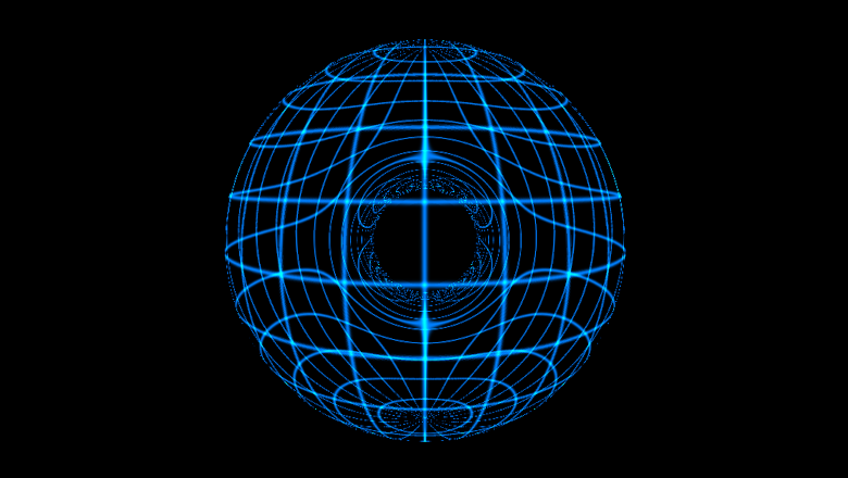
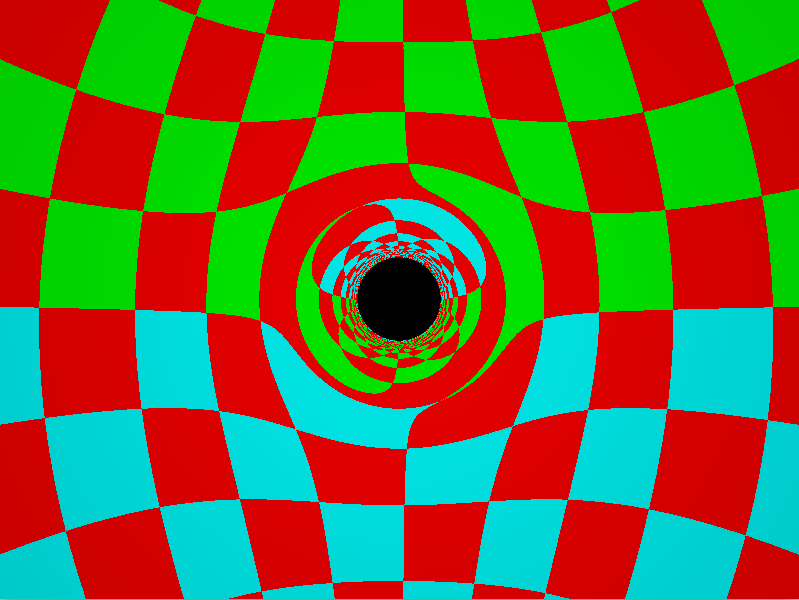
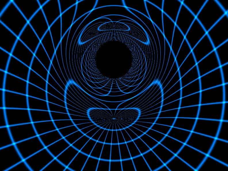
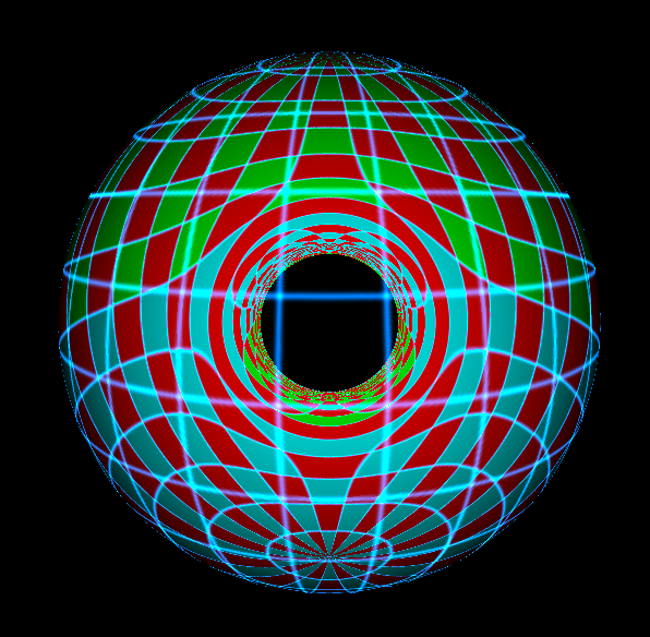
The camera is placed inside a colored spherical shell surrounding the black hole. Rays are traced backward in time from the camera through each pixel. The result shows dramatic gravitational lensing: light from the shell's surface is bent by spacetime curvature, producing image doubling near polar regions and the characteristic distortion of the event horizon vicinity.

Performance bottlenecks appear near coordinate singularities, but the implementation is fully functional and demonstrates practical application of differential geometry concepts on modern GPU hardware.