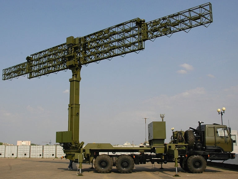
Radars and How to Hide from Them. Part 5: Modern Radars

In the first, second, and third parts of our conversation about radars we discussed the history of their emergence and rapid development during World War II, and in the fourth part the appearance of anti-aircraft missiles and the associated development of radars and countermeasures. In this part we will discuss modern radars and surface-to-air missile systems.

Self-Guided Missiles and Target Illumination Radars

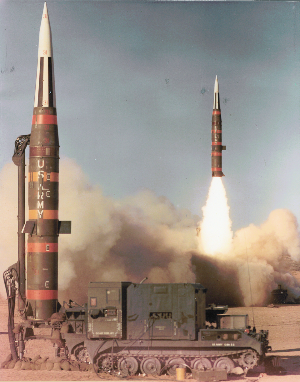
All the anti-aircraft missiles we have discussed so far were "guided" to their target by a system located outside the missile itself. This made the design cheaper and simpler, but the price paid was inevitably rather low guidance accuracy that also worsened with distance. To ensure an acceptable probability of hitting a target even at a range of 40 km required warheads weighing 100–200 kg. At a range of 120 km, as we recall, the Americans resorted to using nuclear weapons, and where this was impossible they used a monstrous 500 kg warhead. Naturally, missiles that had to "carry" such monsters were themselves quite large — they were difficult to fit even on ships, let alone on aircraft.

The reduction in missile size that the military demanded from scientists required a reduction in warhead size. To maintain acceptable effectiveness of a small warhead, the missile's guidance accuracy had to be improved by an order of magnitude. This was achieved only by placing the guidance system on the missile itself (a "homing" system). With homing, as the missile flies it effectively brings its radar closer and closer to the target, and the shorter this distance the higher the accuracy of determining the target's position. While old anti-aircraft missiles with radio command guidance had accuracy measured in tens or even hundreds of meters, homing missiles typically miss by no more than ten meters despite using significantly more primitive radars that must fit within the very compact dimensions of the missile.

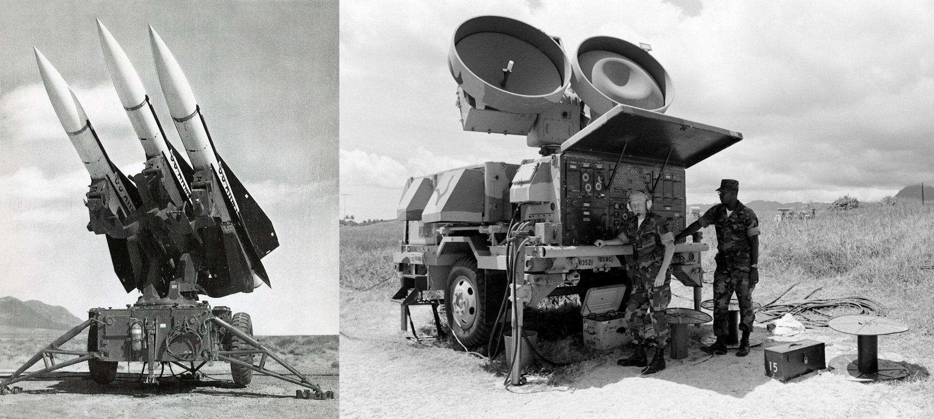
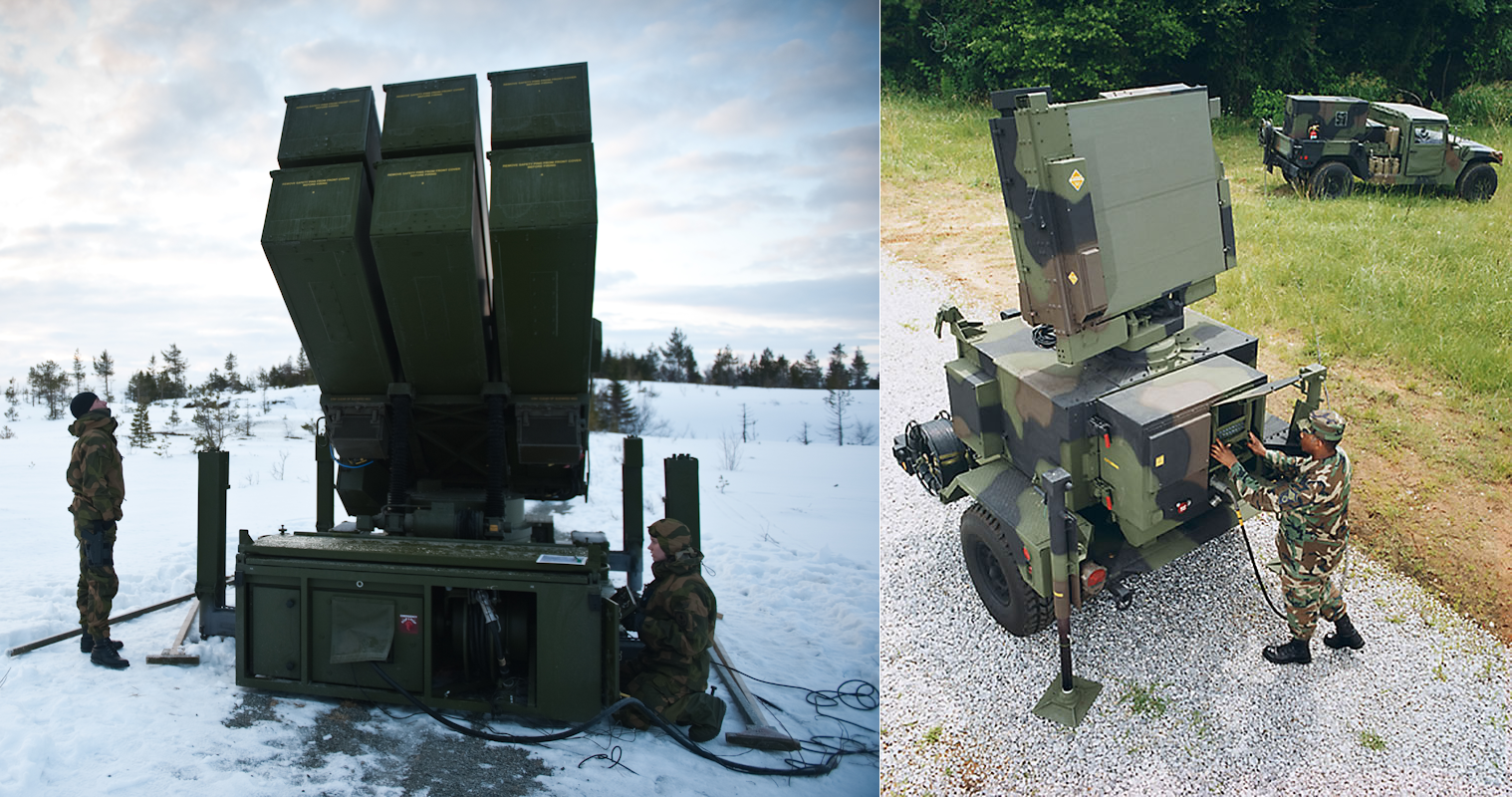
From the moment of their creation to the present day, most anti-aircraft missiles with radar homing use so-called semi-active homing systems (SARH — semi-active radar homing) where only the radar receiver is on the missile, while its transmitter (the target illumination radar) remains on the launching system. This significantly reduces the complexity and cost of the missile while maintaining high guidance accuracy.

Conceptually, a SARH system is in some ways even simpler than command-guided missile systems. The target illumination radar works as a "spotlight" in the radio band, emitting a signal toward the target. The signal reflected from the target forms a kind of "radio beacon," and the receiver on the missile simply has to track this beacon:

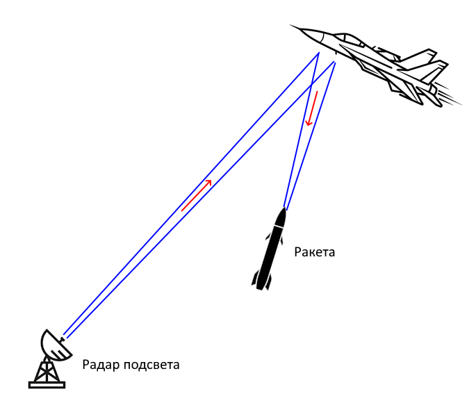
As a rule, the illumination radar has a very narrow beam pattern and continuously tracks the moving target — this significantly increases signal power in the vicinity of the target and consequently the return echo that the missile can "hear." Moreover, the emitted signal is typically not pulsed but continuous — this also increases signal power at the missile's receiver and simplifies the homing scheme. In the simplest variant, a single receiver and antenna are placed on the missile, "looking" slightly off the missile's axis. By spinning this system along the missile's axis (sometimes along with the missile itself) we immediately get the "conical scanning" system already familiar from Part 2. All that remains is to connect the output of its control signal to the missile's steering actuators — and the homing system is ready. Systems built on this principle continue to be used today.

The problem with such simplest systems, however, is that they implement the "pursuit method" which, as already mentioned, forces the missile to maneuver quite strongly, especially in the final moments on head-on courses when the target moves relative to the missile at high angular velocity. Because of this, the miss distance in many scenarios turns out to be quite large, largely negating the advantages of homing. Counter-missile maneuvers exploiting this vulnerability by maximizing the aircraft's angular velocity relative to the missile were naturally developed. However, in the early 1950s the Americans invented a more sophisticated system called "proportional navigation" (proportional guidance) that completely fixed this drawback:

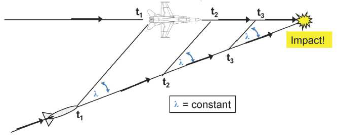
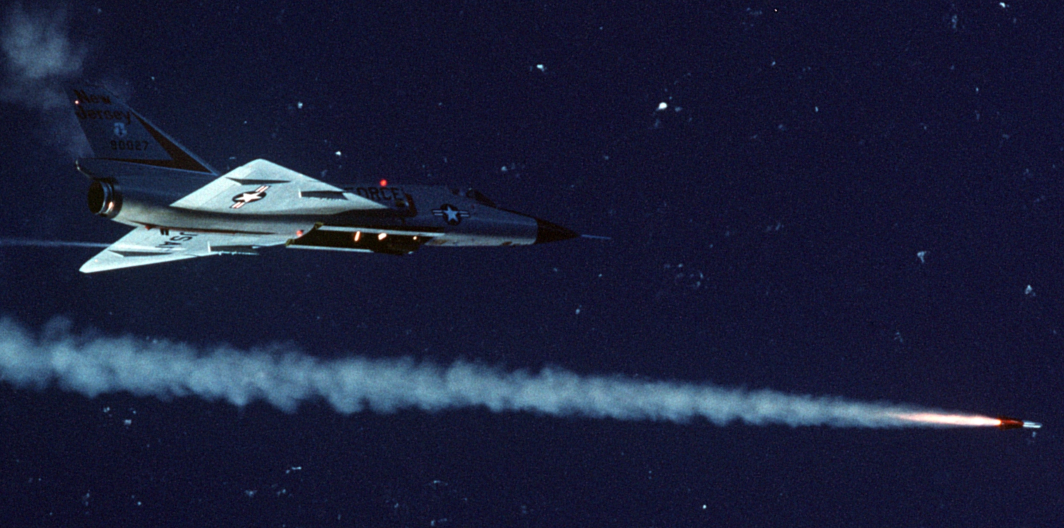
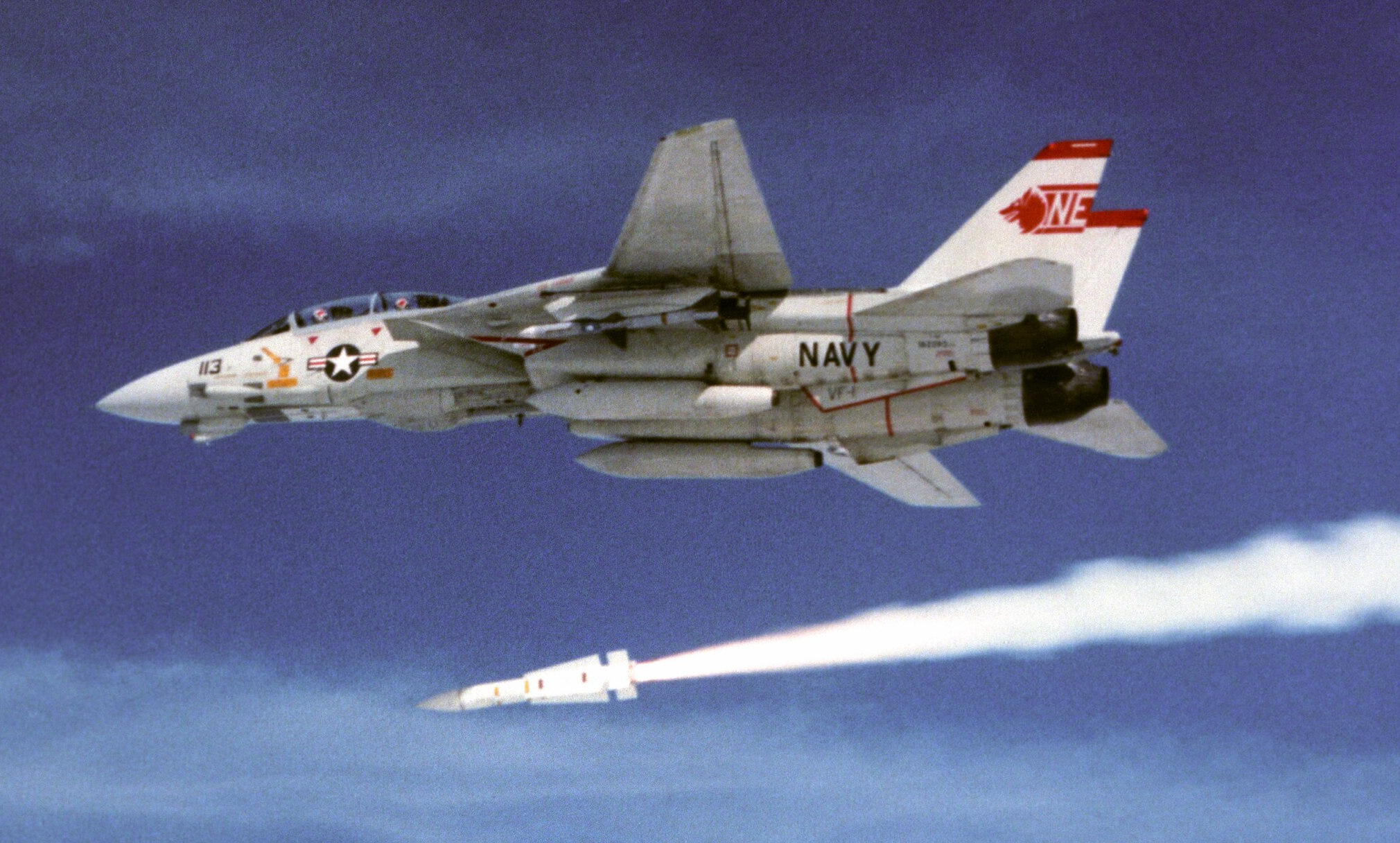
Fundamentally, it is based on an idea well known to sailors: if two ships are moving on a course that will lead to collision, the second ship appears stationary from the first, simply growing ever larger. If the ship visually shifts left or right, there will be no collision. Mathematically, this is illustrated by the picture above — all three triangles are similar and therefore the marked angles (direction to target) are equal. In proportional navigation systems, the seeker head (antenna or entire radar) can rotate relative to the missile and is controlled so as to always remain pointed at the target while the missile itself may be flying in a different direction. The missile's control system tracks the angle between the missile's axis and the seeker head's axis, or more precisely the rate of change of this angle (angular velocity). If this rate is zero, the missile is moving toward the right point. Otherwise, the missile should begin rotating in the opposite direction to compensate for this angular velocity. For this, the missile's control surfaces are deflected by an angle proportional to the measured angular velocity — hence the method's name. The method was first applied on AIM-9 Sidewinder missiles with infrared seekers and proved so successful that, despite its relatively high cost, it effectively displaced all other guidance methods everywhere except for the cheapest missiles.

Systems with semi-active homing and proportional navigation today remain the most popular way to implement SAM systems. However, practical combat experience has shown that their main disadvantage is the need to continuously track the target with the radar beam right up to the moment of missile impact. This creates many options for countering such systems.

First, the aircraft being fired upon receives early warning from its RWR (Radar Warning Receiver) that a missile has been launched and can try to maneuver out of the engagement zone.

Second, the illumination radar gives away its position and an anti-radiation missile can be immediately launched at it, putting its operators before a choice between "try to hit the aircraft but risk losing the radar" or "turn off the radar and try to evade the missile but certainly miss the aircraft." Both these problems are especially acute for "long-range" systems where the missile's flight time can be quite long.

The third major disadvantage of semi-active homing is the need for a special "target illumination mode" on the radar or even an entirely separate radar. In both cases, the radar during missile launch can only track a single target (though simultaneously guiding any number of missiles at it). If you want to shoot at three or four different targets simultaneously — install three or four separate illumination radars.

One possible partial solution to this problem is combining homing and command guidance systems. The launched missile initially flies using good old command guidance technology and only activates its homing system on approach to the target. In this variant, the RWR may fail to recognize the launched missile in time, and the illumination radar can manage to illuminate several different targets in succession while not transmitting long enough to be targeted by an anti-radiation missile. However, such systems are significantly more complex to implement and don't always solve all problems. Therefore, as radars miniaturized, some missiles began receiving so-called active seekers that include not only the radar receiver but also its transmitter. The missile can then be fully autonomous — "fire and forget." This greatly increases the survivability of platforms launching such missiles: they essentially only need to switch on for a few seconds to launch, after which they can immediately retreat from return fire. However, the range of the small radar on the missile is in practice quite limited: there is always a risk that it simply won't be able to "acquire" the target. Therefore, such systems are usually supplemented with inertial guidance (the missile initially flies blindly "somewhere in that area" and only then activates its radar) or command guidance (periodic corrections are transmitted to the missile about where it should fly).

Initially, missiles with active homing were limited to long-range air-to-air missiles where the advantages of this method are greatest, but today they are gradually becoming more widespread. The launchers for such missiles are maximally simple and cheap (though the missiles themselves are not) and are convenient for hiding to work "from ambush"; there are practically no limits on the number of simultaneously engaged targets, and the RWR can only give warning a few seconds before missile impact.

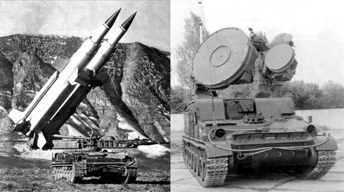
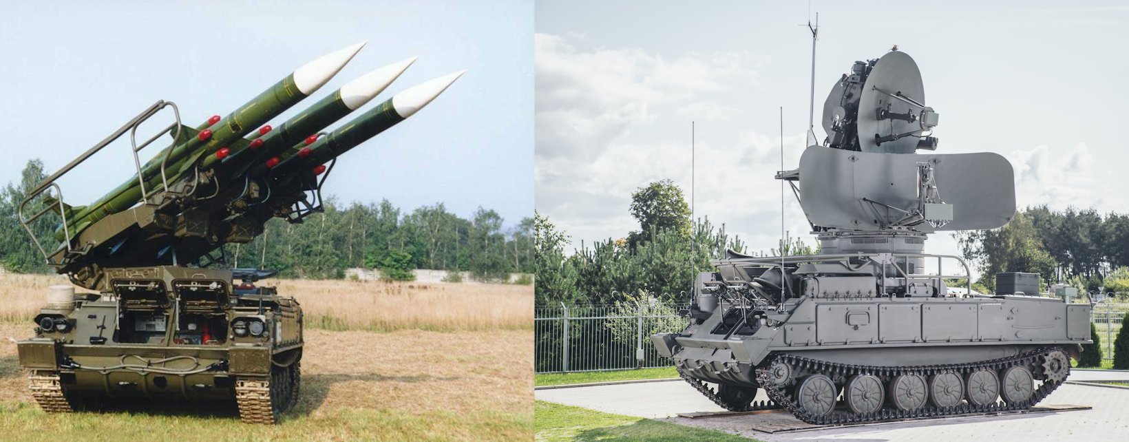
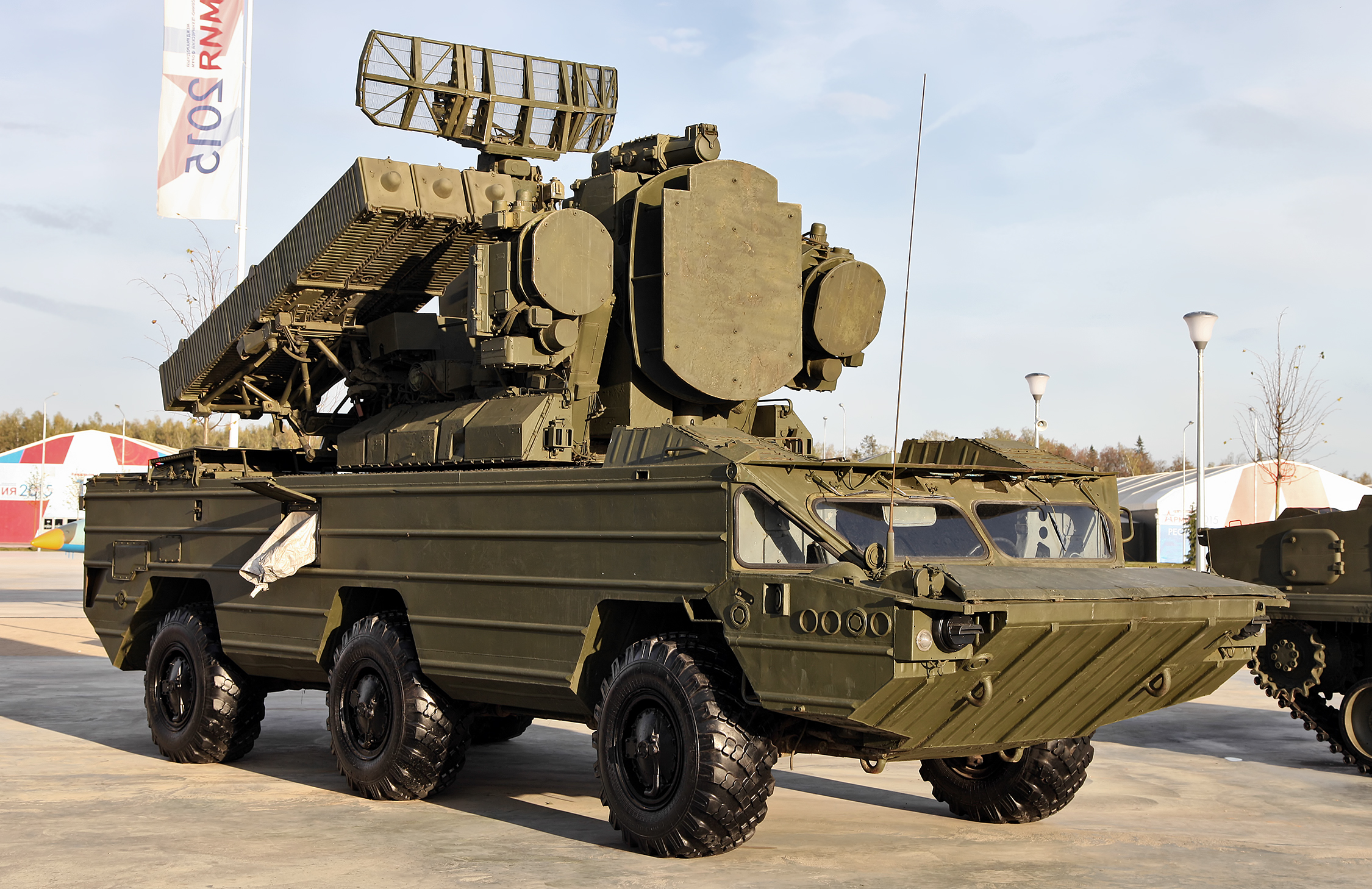
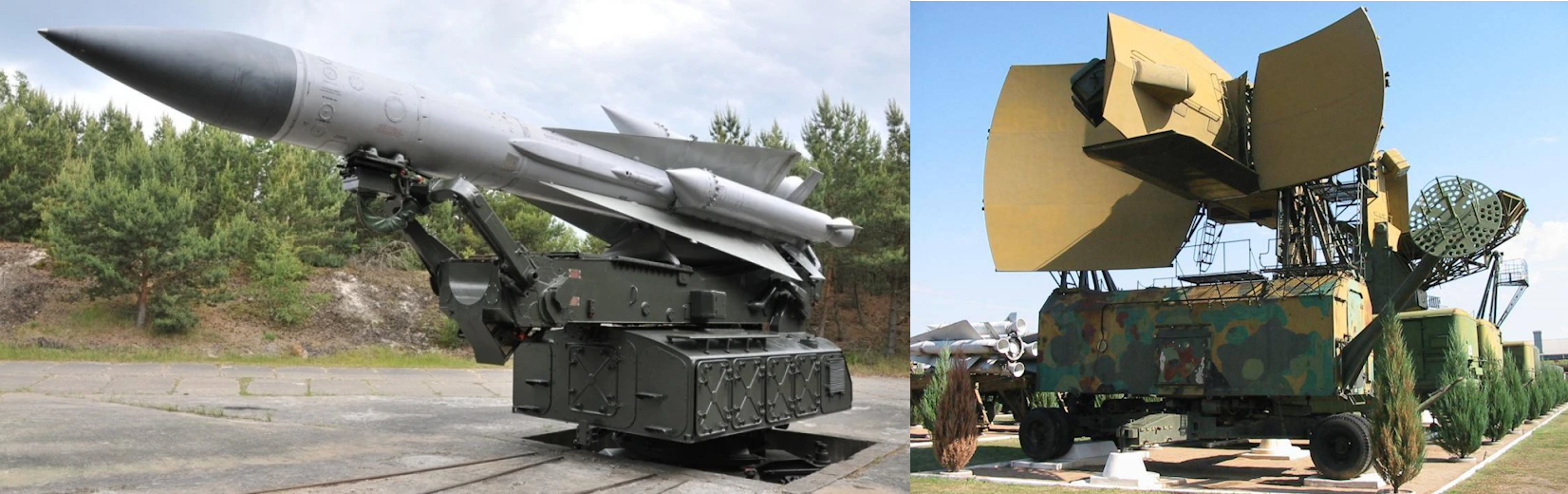
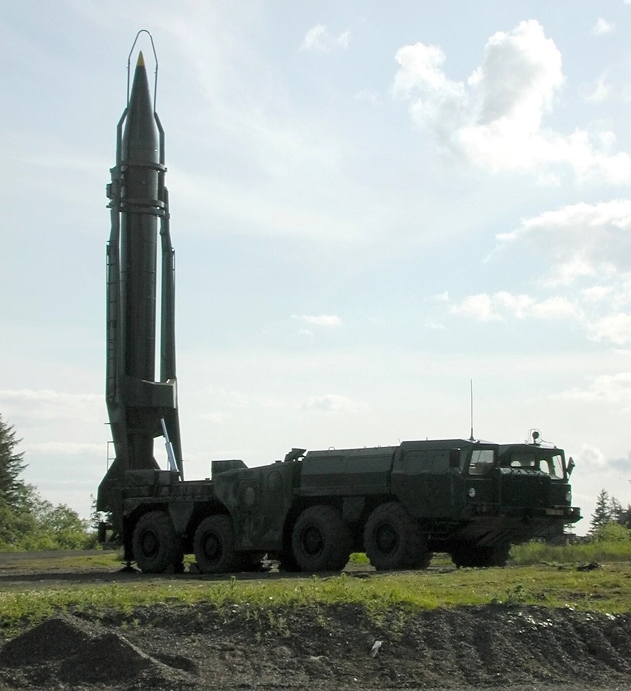
SAM systems with radio command missile guidance, however, haven't disappeared entirely either. They have been pushed into the area of short and very short range systems where the drop in radar accuracy with distance is not yet too noticeable. A classic representative of this family is the Osa SAM system with a firing range of up to 10 km:

The advantage of such systems is the ability to control the missile via television in situations where the adversary manages to suppress radar operation. And this happens not so rarely — fitting a sophisticated radar into a missile is difficult, and a human capable of manually filtering interference is simply impossible. However, simply "jamming" a missile with semi-active or active homing is useless — it will effectively home in on the radio signal source. One must use "smart" jamming systems that disrupt homing with "deceptive jamming" that creates a false impression in the missile that the target is somewhere else by exploiting vulnerabilities in the target-direction-finding algorithms.

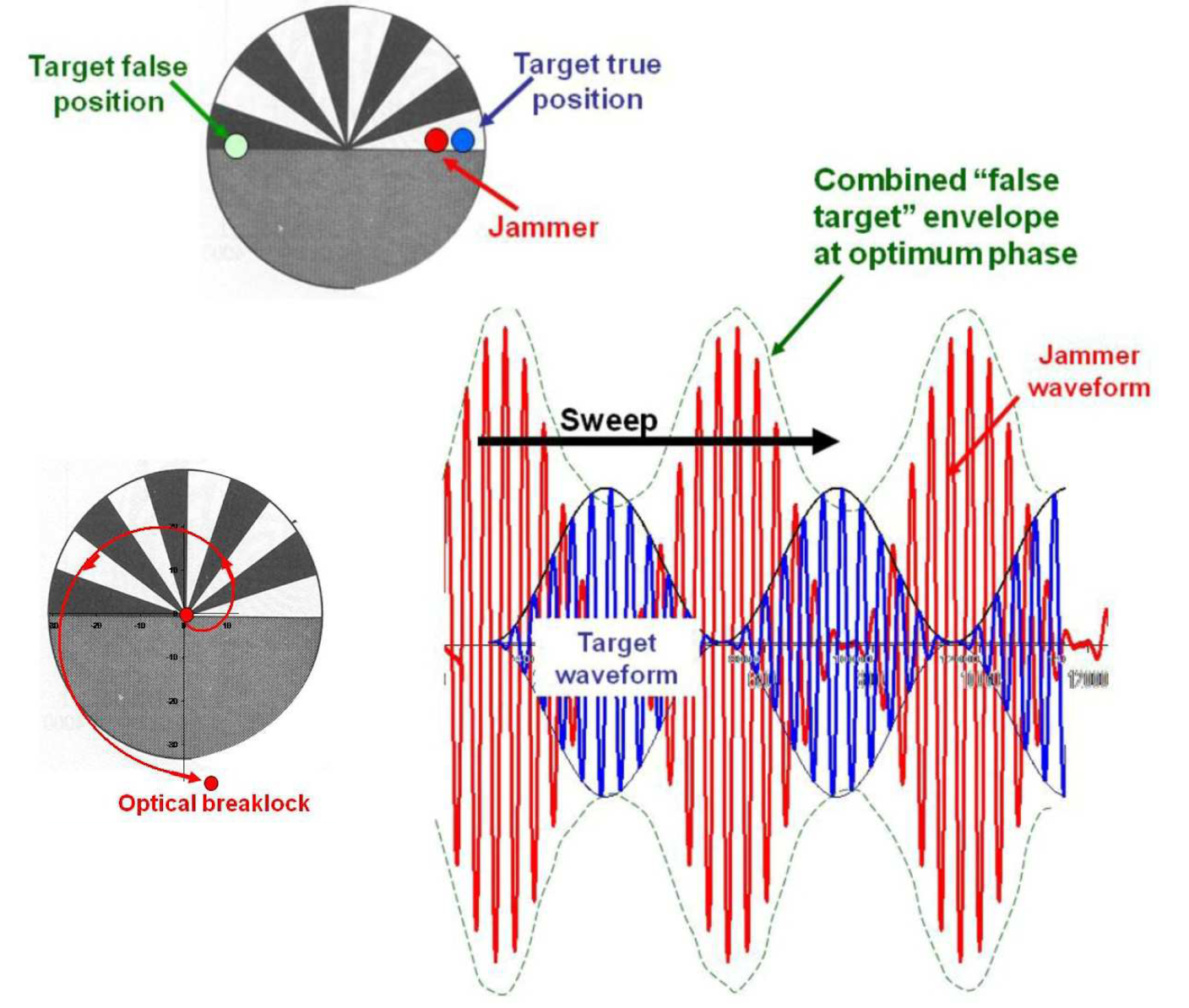
Since this requires precise knowledge of how a particular missile model functions, modern EW (electronic warfare) stations installed on aircraft are essentially computers with extensive databases whose task is to automatically identify the type of missile launched at the aircraft from its radio signal and deploy the appropriate countermeasure. This of course makes knowledge of how the adversary's systems work critically important, which brings us to the next topic —

Coded Pulses and Signal Compression

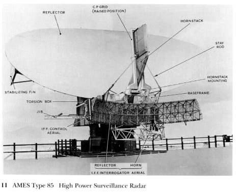
For a long time, radars used very simple signals — one frequency, modulation at best with rectangular pulses at equal (or nearly equal) repetition rates. But alongside them, almost from the very beginning, there existed identification friend-or-foe (IFF) systems whose task was to generate complex coded signals that allowed distinguishing "friendly" signals from "hostile" ones and changing the "recognition code" relatively easily when necessary. The use of coded pulses in radar sharply hampers the adversary's ability to spoof them. However, making a system with complex signal coding was only achievable for a very long time at relatively low frequency ranges. Therefore, initially the radar's "secret code" was simply its operating frequency. Many radars were designed so they could be switched fairly quickly between different frequencies, and some of these frequencies were deliberately not used in peacetime to keep them secret. For example, the British Type 85 radar could switch between 60 different frequencies, of which only a third were used in peacetime. This is called the radar's frequency agility.

But if we can quickly switch between different frequencies — what prevents us from doing this literally with every pulse of the radar? Then even an adversary actively listening to the airwaves won't be able to guess what frequency the next pulse will be on and won't be able to set up the corresponding jamming. This is called frequency hopping. In surveillance radars where the transmitter and receiver are on the same installation, the frequency can change in a truly random manner, but more commonly systems are used where frequency switching occurs according to a specific sequence of frequencies known in advance, which allows synchronizing transmitter and receiver operation even if they are in different locations (for example, the receiver is flying on a missile). Usually such a sequence is generated from a secret key using a pseudorandom sequence generator. In this case the method is called FHSS — frequency hopping spread spectrum.

Beyond radars, this technique has gained widespread use in communication systems since it turned out that jamming (or eavesdropping on) military communications often has no less powerful an effect than suppressing radar operation. Using FHSS forces the adversary to jam a wide frequency band to interfere with narrowband transmission, expending far more energy on jamming than the radio spends on transmitting useful data. It also greatly hampers signal eavesdropping and spoofing. Interestingly, after military adoption, this same method later found application in civilian radio communications where unintentional "interference" comes from household noise sources and other radio stations operating in the same frequency band.

Besides frequency hopping, other ways to hinder effective spoofing of radar signals include varying pulse duration (if the echo is too long or too short, the radar can identify the target as fake) or aperiodic transmission (many systems need to know the moment of radar pulse emission — otherwise their response pulse will arrive "too early" or "too late"). Another interesting method is the simultaneous use of several frequencies by the radar at once, which expands the number of possible variants for each individual pulse. But all these methods are used less frequently — fast (pseudo)random frequency hopping gives the same or better effect, and methods that can cope with it can also cope with duration changes and aperiodic pulses.

Yet another very interesting method of protecting a radar from signal "spoofing" is Doppler shift verification. As we discussed in previous articles, objects moving toward or away from the radar introduce tiny changes in the reflected frequency. In previous articles we focused on using these changes to filter out echoes from stationary objects, but digital echo processing allows the radar to determine from the periodic change in signal "brightness" at the output of the phase detector not just the presence but the exact value of the Doppler shift. Since the Doppler shift shows the target's radial velocity, the computer can predict the next position of the radar signal by range and its phase. And if the mark appears at the correct distance — it's genuine, and if not — it's fake. This method not only forces the jamming system to account for the Doppler shift but also requires knowing the radar's position, since radial velocity depends on the relative positions of radar and target.

The Doppler method works especially well for continuous-wave radars. As we discussed in previous parts, determining the Doppler shift in a single pulse is difficult and requires non-trivial radio engineering. But in continuous-wave radars, the received signal is so monochromatic that determining the exact frequency shift poses no great difficulty even in an unsophisticated missile warhead. Therefore, many simple ECCM (electronic counter-countermeasures) methods for semi-active and active homing missiles include transmitting the calculated radial velocity of the target relative to the missile and narrowband filtering tuned to this specific radial velocity. To effectively suppress such a system, the jammer must correctly determine the missile's radial velocity.

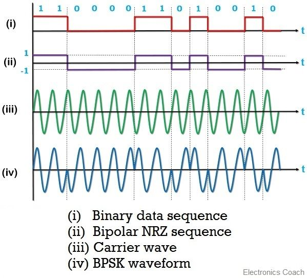
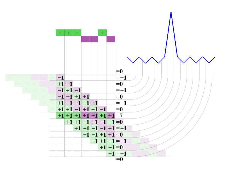
Another very interesting method is phase-shift keying (PSK) of the radar signal. In this mode, the radar transmits a continuous signal on one frequency but essentially breaks it into a chain of short sub-pulses following directly one after another, each of which may differ in phase:

The radar's receiver can decode the phase sequence in the received "echo" and compare it with the transmitted signal. In older "pre-digital" systems, this was often implemented through a chain of several delay lines that create several copies of the signal delayed by multiples of one "sub-pulse" duration. Then the phase in these copies is shifted by the opposite of the phase shift in the code, and everything is summed together:

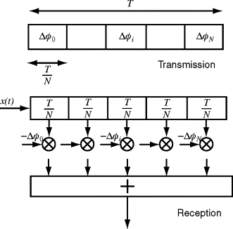
If the signal is received correctly, the phases of all delayed copies will after such rotation be turned "in one direction" and the signal will add up and mutually reinforce. If the signal doesn't match the pattern, some phases will be turned "in the opposite direction" and when summed will reduce the signal magnitude. Mathematically, such a filter implements the convolution operation of the signal with the code sequence. With a "good" code choice, the useful signal at the filter output hovers near zero even at the moment of receiving real echo until the moment of perfect match, producing a short signal peak, after which the signal again effectively "mutually cancels." This is called pulse compression — the peak signal at the receiver output turns out much shorter than the duration of the original sequence in the phase-shift keyed signal:

Interestingly, such coded pulses are used not only in radars but also in telecommunications systems for synchronization signals. There is an entire theory devoted to efficient generation of such signals with "good" autocorrelation functions, but it deserves a separate article. As applied to radars, it suffices to know that a) such a scheme provides certain protection against jamming and b) it "compresses" the received pulse in duration while proportionally increasing its amplitude. The second property is used far more today than the first because it solves the old dilemma of all pulsed radars: short pulses provide high range accuracy but poor noise immunity, while long pulses provide good noise immunity but poor accuracy. Encoding a long pulse as such a series of short "sub-pulses" provides received signal strength at the level of a long pulse and spatial accuracy at the level of a short pulse.

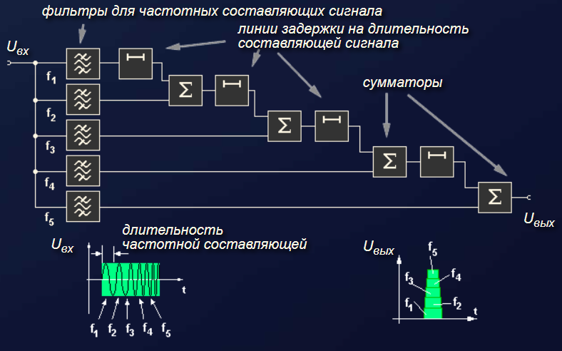
Phase coding is not the only possible pulse compression scheme. Any schemes that break the signal into several pieces that can be detected separately will work. For example, in radars with frequency hopping, one can send a sequence of pulses on different frequencies or use a control scheme providing linear frequency modulation (chirp). In the receiver, instead of phase shifters a chain of filters for different frequencies is installed. The principle is similar — at each filter's output the received echo forms a short response with some delay, and these signals are summed so that these delays compensate each other. The result is a scheme where the output from all filters when receiving a "correct" echo adds up and reinforces each other.

The development of digital signal processing systems sharply simplified the creation of such systems and led in the 20th century to the emergence of extreme variants where the signal is formed as sequences of many hundreds of thousands of such "sub-pulses," often combining both frequency and phase manipulation. The signal becomes so super-long that it is practically indistinguishable from continuous, yet its decoding produces an extremely narrow and very powerful pulse. In addition to enormous noise immunity, such signals are good because they can be made very weak — instead of short pulses of kilowatt power, the radar can continuously emit just a couple of watts of radiation and achieve the same results. This is called LPIR — low probability of intercept radar. The low emission power of such a radar and a signal that resembles ordinary noise greatly hamper its detection.

Besides schemes that break individual "large" pulses into "mini-pulses," modern radars also typically implement signal "accumulation" schemes. In old radars, as I already wrote, such "accumulation" was often achieved through the persistence of screen phosphor and human vision — the visible signal on the screen was brighter where it continuously repeated. In modern radars, similar results are achieved by digital signal processing. Averaging a sequence of N pulses allows amplifying the signal by √N relative to random noise, and with a sufficiently high pulse repetition rate or sufficiently long observation of the target, even a very weak signal can be extracted. However, unlike pulse compression schemes, signal "accumulation" must account for the fact that the object may move through space.

The most advanced schemes with long digital sequences (such as LPIR) are typically designed so that their emitted signal is essentially continuous, but can be interpreted as a continuous sequence of pulses. For this, the signal is designed so that in a very long code sequence any desired "substring" can be effectively and unambiguously found. Using digital processing, we can essentially just "cut out" that piece of signal and effectively separate it with a filter from the rest of the sequence. At the same time, we can "slice" the signal into any number of pieces, including overlapping ones. This scheme is most familiar to us from GPS signals, which essentially implement "radar in reverse" where we determine distance to a moving satellite from the delay in the received signal, and from distances to several satellites with known coordinates we determine our own position.

The signal emitted by GPS satellites is just 50 watts spread over half the Earth's surface, so its power at the Earth's surface is on the order of 10⁻¹⁴ watts per square meter, or in units more familiar to radio amateurs, −135 dBW. For comparison, the signal from ordinary cell towers is −45 dBW under ideal conditions (i.e., 10⁹ times stronger), and when it drops to about −110 dBW (300 times stronger than the GPS signal), the cell signal is no longer received by the phone. In fact, the GPS signal is so weak that it is 100 times below the level of natural noise coming from space. The tiny antenna of the receiver in your phone doesn't exactly help reception quality either — its input power is measured in fractions of a picowatt (on the order of 10⁻¹⁶ W). Add to this the cosmic speed of satellites moving through space at kilometers per second. Nevertheless, as we know, GPS receivers work excellently — and this is perhaps the most vivid illustration of the incredible capabilities of modern radar technology. Just 1 second of GPS signal measurement gives a bit sequence 10 million samples long, sufficient to amplify the signal approximately 3,000 times compared to noise, and this turns out to be enough to reliably detect it with a time error significantly less than the length of one sequence pulse. The capabilities of modern military radars are classified, but it is known, for example, that similar digital schemes were used for such stunning projects as radar mapping of Mercury's surface (at a range of over 100 million km!) using the Arecibo Observatory.

Secondary Surveillance Radar

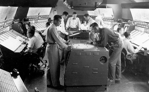
The modern world is inconceivable without air transport. Whether passenger flights or cargo — today at any given moment there are on average 12,000–14,000 aircraft in the air worldwide and about 1 million people. In the early days of civil aviation, when the number of flights in the US was still only a few hundred per day, pilots flew independently and relied on visual identification to avoid hitting anyone. But in the first decade after World War II, civilian traffic grew 25-fold, exceeding railroad traffic in America by 1955. In major aviation hubs like New York, arrivals separated by just a few minutes became common. At the same time, aircraft speeds had increased significantly, and the development of navigation aids made safe flights possible not only in good weather.

The natural consequence of the growing number of aircraft, their speeds, and increasingly frequent flights in dense clouds was a rise in midair collisions. Moreover, practice soon showed that not only civilian aircraft collided with each other, but military ones too. It was obvious that the situation would only worsen. The response was the creation of standardized and unified national air traffic control systems that replaced the earlier civilian dispatchers who controlled only individual busy points. The new systems took over management of both civilian and military air traffic. And thanks to radars, controllers no longer relied on reports from pilots themselves, whom previously had to be periodically queried by radio to clarify their current positions. From 1958–1960, the US and Europe saw mass implementation of flight rules under controller supervision, and airspace was divided into "zones" and so-called "classes" depending on how strictly flights were controlled and who was responsible for control.

The first experiments using radars for air traffic management began back in 1948 but were initially limited to short-range radars controlling the arrival and departure zone in the immediate vicinity of the airport. In 1952, the first "civilian" radar designed for these purposes appeared — the ASR-1. Interestingly, its initial use met fierce resistance from pilots who didn't like controllers "watching" to make sure they were flying correctly. As controlled airspace expanded, longer-range military early warning radars were also applied to tracking civilian flights.

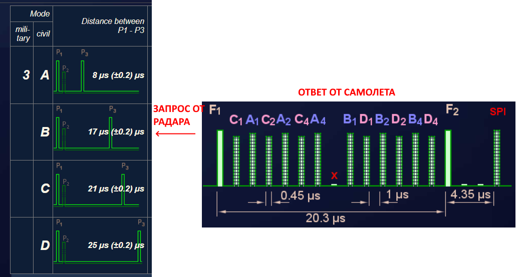
However, using "military" radars was inconvenient in many respects. First, it required fairly close coordination with the military and was a potential source of "military" information leaks, such as (for example) radar maintenance downtime schedules. Second, military radars were problematic to supply to third countries, and air traffic was rapidly becoming international. Therefore, from 1954 the International Civil Aviation Organization (ICAO) set about standardizing a more practical Secondary Surveillance Radar (SSR) system for tracking civilian flights. Unlike ordinary "primary" radar where the aircraft passively reflects a radio pulse echo, in "secondary" radar systems the response to a received radar signal is sent by an active system — a transponder. As I already wrote in earlier articles, the international standard was based on the already existing obsolete military identification system Mark X, specifically one of its sub-modes — Mark 3. This was convenient because it ensured compatibility with existing military systems and correct recognition of civilian aircraft by military systems (and vice versa). In response to a received sequence of two or three pulses (P1, P2, and P3) with strictly defined intervals between them, a civilian aircraft's transponder was to send a series of up to 15 pulses. This included start and stop bits (F1 and F2) at specific positions, a "dead" bit where there should be no signal (to effectively reject incorrect data transmissions), and 12 bits of actual "payload."

In early systems, only the so-called "Mode A" was defined, in which the aircraft sent its identification code (SQUAWK) in the 12 bits. Due to the use of an active transponder, signal power in such a system falls with distance only proportionally to 1/d² rather than 1/d⁴ as in ordinary radars, so it became possible to fairly easily create cheap and compact radars with a range of 400 km. Additionally, these radars didn't receive parasitic reflections from the ground and consequently didn't require complex and expensive MTI systems. Their operating logic initially completely replicated that of military radars — a rotating antenna formed a narrow beam in which a continuous sequence of pulses — "interrogations" — was sent, and upon recognizing them the aircraft's transponder was to send its identification code with a strictly defined delay. From the delay of the received response, the receiver determined the distance to the aircraft; from the antenna's azimuth angle — the approximate direction. There was no need to aim missiles at civilians, so accuracy of a kilometer or two initially satisfied civilian controllers just fine. From 1960, transponder installation became mandatory for all military and civilian aircraft in the US.

However, as secondary radar systems saw wide practical use, problems emerged that ordinary radars typically didn't have. For example, it turned out that at sufficiently close range the radar's signal (designed to trigger at 400 km range) was strong enough for the transponder receiver to recognize it even when the radar antenna was pointing "the other way" from the aircraft. In turn, the response signal was often also strong enough for the radar to receive it. In the worst case, the secondary radar would receive signals from the aircraft regardless of which direction the antenna pointed, forming instead of a single point on the screen an entire ring at a certain radius from the radar. If the problem was less critical, instead of dots the marks on the radar screen turned into arcs, or false targets appeared in the directions of the antenna's sidelobes. One obvious way to combat this was improving antenna directionality, but later a simpler and cheaper solution was found. An omnidirectional antenna was added to the radar design that, when the radar emitted main interrogation pulses P1 and P3, transmitted an additional pulse P2 in all directions (see the figure above). The strength of the P2 signal received by the transponder allows its receiver to estimate the distance to the radar and distinguish between the situation where the received signal is weak because the distance to the radar is large and the situation where it's weak because the radar antenna is pointing elsewhere. For this, the receiver simply compares the signal levels of P1 and P2 and transmits a response only if P1 is significantly stronger than P2. This allows cheap and effective suppression of identification signal transmission outside the main lobe of the antenna pattern.

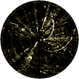
The second problem related to high signal power was... FRUITs, or more precisely FRUIT interference — False Replies Unsynchronised to Interrogator Transmission. Due to the long range of radars, an aircraft often found itself within range of two or more radars simultaneously. But since transponder responses don't depend on which radar sent the query, a radar could register responses to queries sent not by itself but by another radar. Since the interrogation sequences of different radars typically differ, the received signals usually generate not one incorrect mark but an entire "moving" series. This is "fruit." For example, differences in interrogation rates between radars cause the incorrect echo to arrive with gradually decreasing or increasing delay, generating a chain of marks at different ranges. Combined with antenna rotation, this often forms the characteristic spiral visible in the picture above. FRUITs created an especially unpleasant effect before reliable sidelobe suppression systems were created, which provoked aircraft into transmitting large numbers of unnecessary responses. The solution was creating systems of "reverse MTI." In military radars, stationary marks were filtered out (reflections from ground targets), while in civilian radars conversely too-mobile marks began to be filtered — the mark memory scheme began passing only signals received at least twice from approximately the same position.

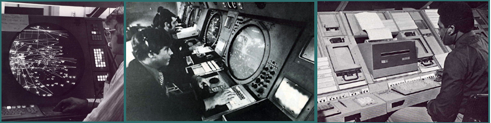
Finally, the third problem was that civilian radars, unlike military ones, initially could only work in 2D, determining direction by azimuth but not altitude. As the number of aircraft grew, it became important to understand whether they would safely separate when their trajectories crossed. Therefore, Mode C queries were added — slightly different from Mode A queries, to which the 12-bit message was to contain the aircraft's altitude. Wide adoption of such systems occurred in the 1970s and coincided in the US with the transition to computer systems that automatically queried aircraft, remembered and tracked their trajectories, could load schedules digitally from floppy disks, and display them. Thanks to "Code C," such systems could automatically warn controllers of possible collisions.

Another interesting feature introduced based on practical experience was the addition of an SPI (selective pulse identification) bit to the transponder response, which was activated for 15–20 seconds when the pilot pressed a special button in the aircraft. This allowed controllers to quickly find the aircraft of interest by transmitting a radio request to the relevant pilot ("Delta 123, press identification button") without needing to manually search for the right mark among dozens of aircraft. All marks received by the radar with the corresponding bit set were highlighted on the screen in one way or another.

As the number of aircraft continued to grow in the 1980s, secondary radar systems were once again modernized with the addition of so-called "Mode S" transponders ("selective"). Mode S expanded the response format from 12 bits to 56 or 112 bits, making possible a) transmission of altitude with higher precision, b) increasing the number of unique identification codes from 12 to 24 bits, and c) simultaneous reception of altitude and aircraft code without needing to make two separate queries and then somehow merge them. But more importantly, it added a similar 56–112-bit data field to the query. Besides enabling the radar to ask the aircraft for a whole range of possible data about its condition (not just altitude), this made it possible to specify in the query the specific aircraft being addressed (hence the new mode's name — "selective interrogation"). Although a Mode S radar can still periodically query all aircraft to understand who is in the airspace, it much more often limits itself to addressing a specific aircraft for data updates. Among other advantages, this solves one problem of earlier Modes A and C — the possibility of overlapping responses from different aircraft:

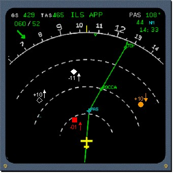
A Mode S radar can simply query aircraft in sequence without overlapping response signals, greatly simplifying things like simultaneous landings of two aircraft on parallel runways. Overall, the sharp reduction in "broadcast" queries sharply reduces the volume of mutual interference between simultaneously operating radars. In particular, this enabled the implementation of aircraft-mounted radars capable of seeing other aircraft: previously this would have created too much interference, but in Mode S this is no longer a critical drawback. On this basis, the first TCAS (Traffic Collision Avoidance System) systems were created, allowing the pilot to see other aircraft and receive warnings of dangerous proximity.

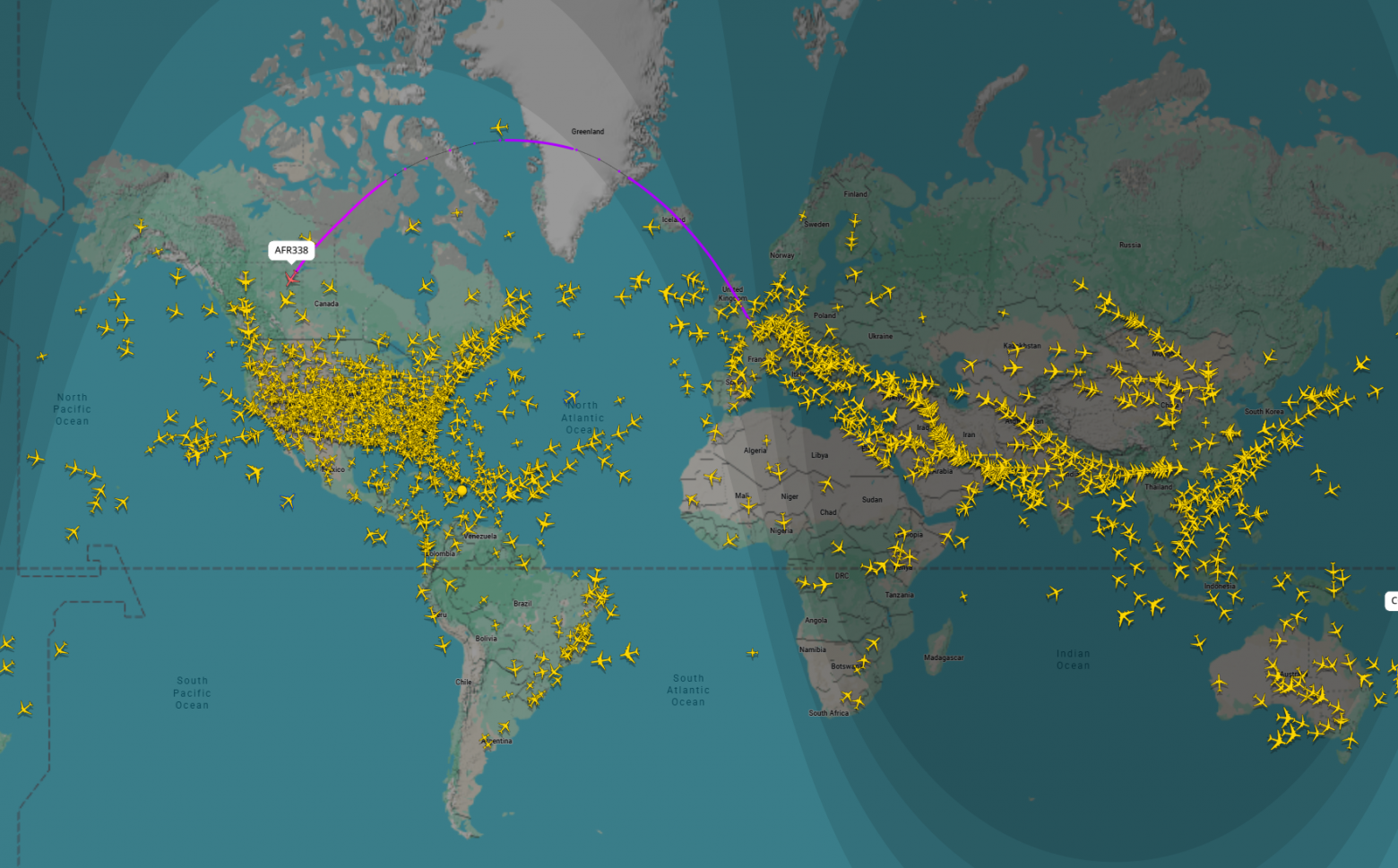
As GPS systems enabling aircraft position determination without radar spread to aircraft, in the 21st century ADS-B (Automatic Dependent Surveillance – Broadcast) was also added to Mode S transponders, which periodically broadcasts into space — without any radar query — a message about the aircraft's coordinates, speed, and flight direction. The advantage of this scheme is that it works literally everywhere — it no longer requires an active radar to see airborne objects around it. Since 2020, this system has become a mandatory standard for the US and will apparently soon become the standard worldwide. And thanks to the fact that ADS-B receivers are today available to any radio amateur, we have sites like flightradar24.com that collect this data from thousands of receivers installed around the world.

Most aircraft today continue to maintain compatibility with older systems like A, C, and S, but older modes will apparently be gradually displaced by new standards.

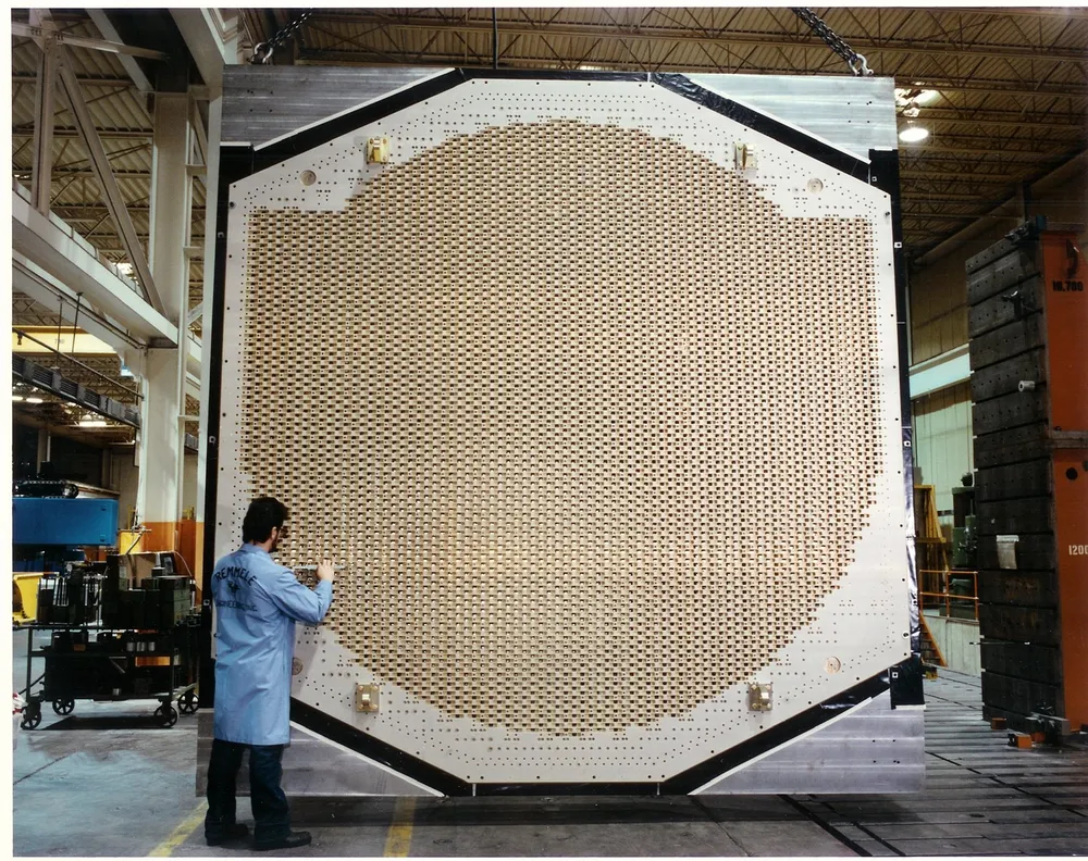
Phased Array Antennas

Another feature of most modern radars is the use of phased array antennas (PAA). Fundamentally, the PAA idea is relatively simple: instead of one directional antenna, we take a set (array) of several relatively omnidirectional antennas, then add a phase delay to each antenna so that the interference of their signals forms a wave directed predominantly in the desired direction.

Signal reception, due to the time-reversibility of radio wave propagation, works exactly the same way — summing signals from antennas with specific delays ensures directional reception. In principle, a PAA can form a signal directed anywhere in space from the antenna array, but for a flat array the efficiency of signal formation drops sharply at emission angles close to 90 degrees from the normal to the plane, and the effective range of emission and reception is usually ±60°.

Historically, the first PAAs appeared because of the reluctance to rotate enormous (and therefore slow or entirely stationary) antennas. In Part 2 we mentioned that the receivers of one of the world's first radars — the British Chain Home (AMES-1) system — worked on exactly this principle. But the efficiency of implementing phase delays using a goniometer at that time was quite poor. As soon as it became possible to reduce antenna sizes to at least several dozen meters, such systems were mostly abandoned in favor of mechanical scanning methods (antenna rotation). The scanning speed of these methods was often far from slow. In the previous article we mentioned that the "windmill" of the Soviet S-25 system scanned its sector 5 times per second, and the improved version with a smaller rotating element in the S-75 managed to scan space (admittedly in a much smaller sector) 10 times per second. Systems with parabolic dishes mounted on aircraft performed only slightly worse.

But there's no limit to perfection! As we've mentioned a couple of times, the fundamental problem of the vast majority of early SAM systems was their single-channel nature. At any given time they could only engage one target. The exception was the legendary Soviet S-25, but even it could only engage a 120-degree sector. To provide all-around defense, it would have required installing eight enormous rotating "windmills." The Americans wanted something similar but in a much more compact form that would fit on their ships.

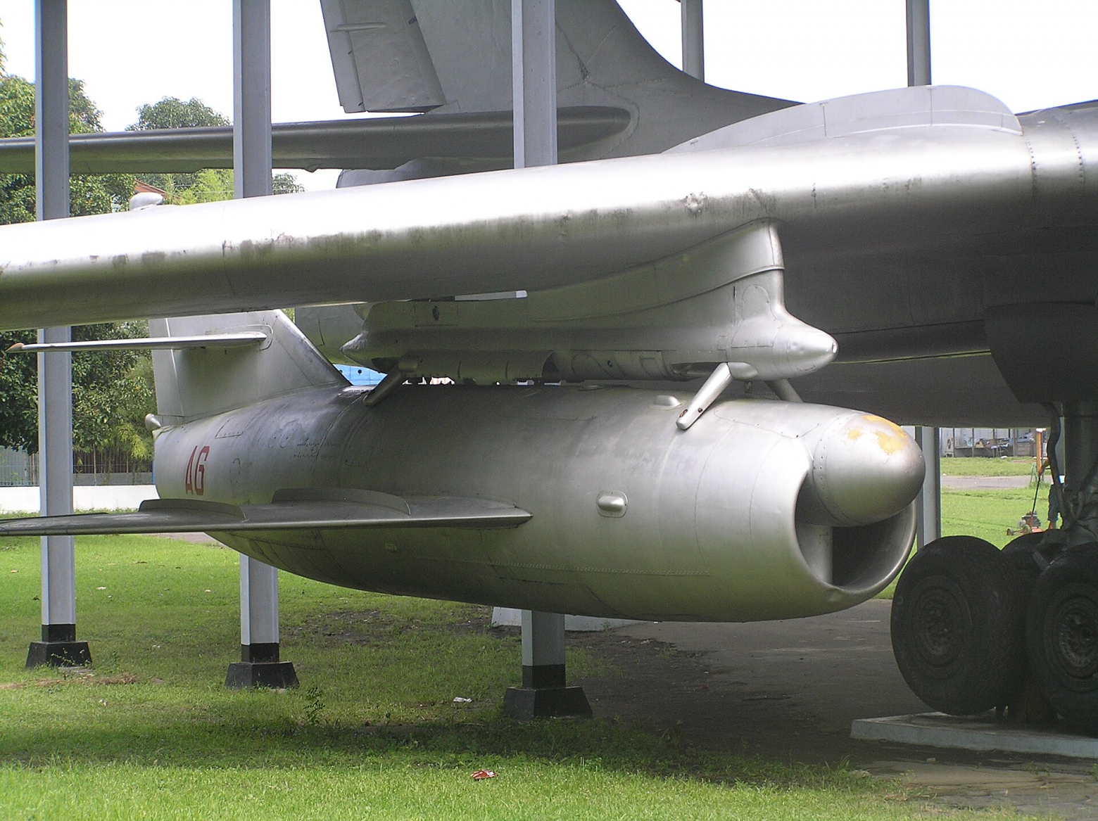
And here we should once again give credit to the USSR. While generally lagging in aviation, they analyzed American experience and created weapons effective against American air defense systems: cruise missiles. Relatively small and fast but most importantly — numerous targets largely replicated the Japanese kamikaze aircraft experience. Initially, they actually resembled real aircraft (MiG-15) — just smaller and without a pilot cockpit.

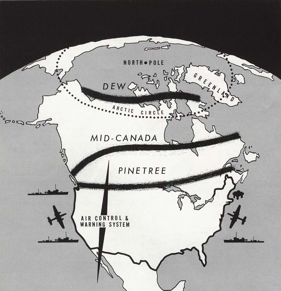
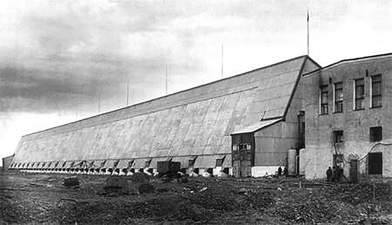
Simultaneous launch of several cruise missiles overwhelmed American air defense capabilities with the number of targets, and the loss of several missiles in a salvo was not as painful as losing the bombers carrying them. The Americans underestimated the threat from this weapon for a very long time, believing they would simply intercept the bombers before they could launch their (initially relatively short-range) missiles. Regarding strategic aviation, this led to the construction of increasingly northern early warning stations whose task was timely detection of Soviet bombers.

But regarding ships, the ability to intercept targets attacking them thousands of kilometers away was initially quite unrealistic, which was ultimately demonstrated in practice by the extraordinarily successful employment of Soviet anti-ship missiles in the late 1960s. A similar problem, but regarding defense of American ground installations, was posed by Soviet short-range ballistic missiles.

Although American SAM systems could theoretically intercept ballistic targets, they couldn't stop a salvo of two or more missiles — and the USSR was banking on precisely the mass employment of such systems. Vulnerable military installations had to be moved farther from possible front lines, which was very inconvenient. Therefore, the Americans faced the urgent question of creating SAM systems capable of simultaneously engaging several targets, some of which could be ballistic. As the Americans adopted the "Soviet experience," similar problems arose for the USSR as well.

Simultaneously engaging several targets with a single radar was proposed by rapidly switching the radar beam between different targets. The radar would illuminate one target for a fraction of a second, update its position, then switch to a second, update its position, then switch to a third, and so on. Between "illuminations," the target's position and speed were stored and interpolated by a computer. For a sufficiently large antenna, implementing this by purely mechanical rotation was impossible. PAAs solved this problem with electronic control of signal phases on a huge number of antennas forming the radiating array (ESA — Electronically Scanned Array).

There are three main PAA design schemes differing in how phase control is implemented in the array.

First, one can place on each antenna element its own separately controlled receiver and transmitter. This is a so-called active electronically scanned array (AESA). In a typical antenna array we're talking about hundreds, thousands, and even tens of thousands of individual elements, making such a scheme traditionally extremely expensive. Moreover, these transceivers must be carefully synchronized with each other, which is also far from simple.

Second, one can use in each antenna a special element called a phase shifter. Typically, the phase shifter is implemented using an electronic circuit that can switch the radio-frequency signal between several conductors of different lengths.

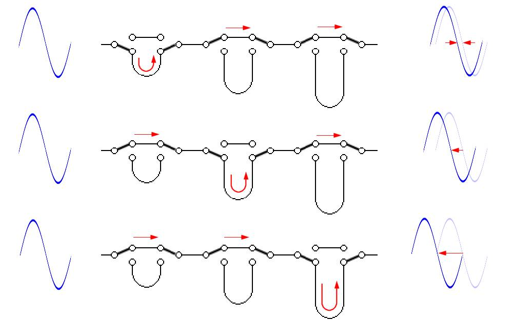
In such a scheme, only one signal transmitter and receiver is used, connected to all antennas in the array, but the desired delay is introduced into each antenna's signal using phase shifters. This is a passive electronically scanned array (PESA) and it is much cheaper to implement.

Finally, there is a third, cheapest variant of electronic PAA implementation: the so-called frequency-scanning array (FSA). Here, fixed-length delay lines are introduced into the antennas, often by simply connecting antenna elements in series with wire segments of the required length. The key is that for a delay line of equal length, the phase shift depends on the wavelength. If a whole number of wavelengths fits in the delay line segment — there is no phase shift. If half-integer — the phase rotates 180 degrees, and so on. By properly selecting delay line lengths, one can make the direction of the signal emitted by the antenna array depend on the frequency of the radio emission fed to it. This type of radar requires a transmitter capable of tuning across a fairly wide frequency range but is generally cheapest to implement.

It should be noted that the beam pattern of any PESA also depends on the wavelength used. This is a fundamental disadvantage of PESA and the main difference from AESA, which has no such limitations. Many PESAs are "tuned" to a strictly defined wavelength they can work with. Others can switch between different wavelengths but cannot work with different frequencies simultaneously. Therefore, wideband PAAs such as Starlink satellite internet terminals can only be active. However, the frequency dependence of PESA is sometimes used as an advantage in combined schemes where beam direction is formed by combining phase shifters for "coarse" antenna tuning and frequency changes for finer "fine-tuning."

I already wrote that individual PAA elements were used during the Korean War in many Soviet radars in the form of "two-story" antennas that could be oriented "by elevation angle" by varying the signal delay between the lower and upper assembly. The Americans were the first to go a step further and create systems combining mechanical scanning in azimuth with electronic scanning in elevation.

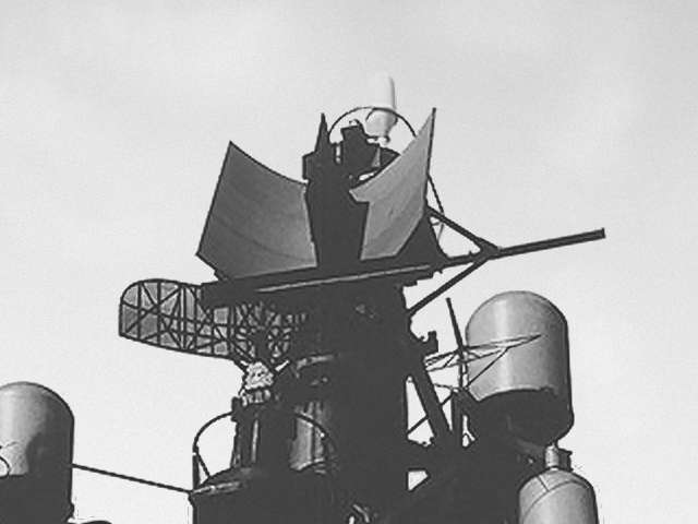
Unlike Soviet radars that simply "tuned" to a certain altitude manually, the American ones scanned space with a rapidly moving beam up and down, allowing determination during one radar revolution of not only all airborne targets around the ship but the altitude of each ("3D radar"). Although by modern standards this is a primitive system, at the time of its appearance it was considered very complex and consequently suffered from low reliability (mean time between failures was initially just 14 hours!). The Americans spent the next 15 years perfecting this approach and improving its reliability.

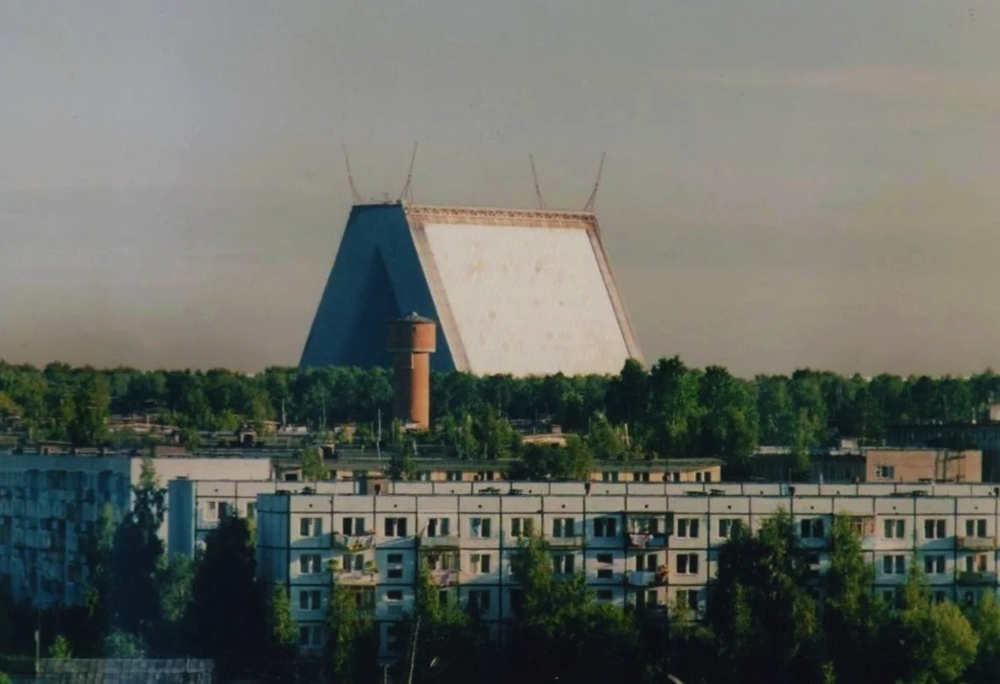
The first experiments with "modern" PAAs with large numbers of antenna elements capable of changing beam direction not only vertically but horizontally also began in the 1960s, but they very long remained within the bounds of experimental models. In addition to the very high cost of such systems due to their high complexity, they also suffered from even lower reliability. Therefore, they initially found real application only in missile defense radars. Due to the need to track tiny missile warheads at distances of a thousand kilometers, such radars inevitably have enormous dimensions and consequently are fundamentally immobile. The ability to electronically control the beam is a forced necessity, and the enormous dimensions allow cramming even quite bulky equipment into the antenna and servicing it with (relative) convenience.

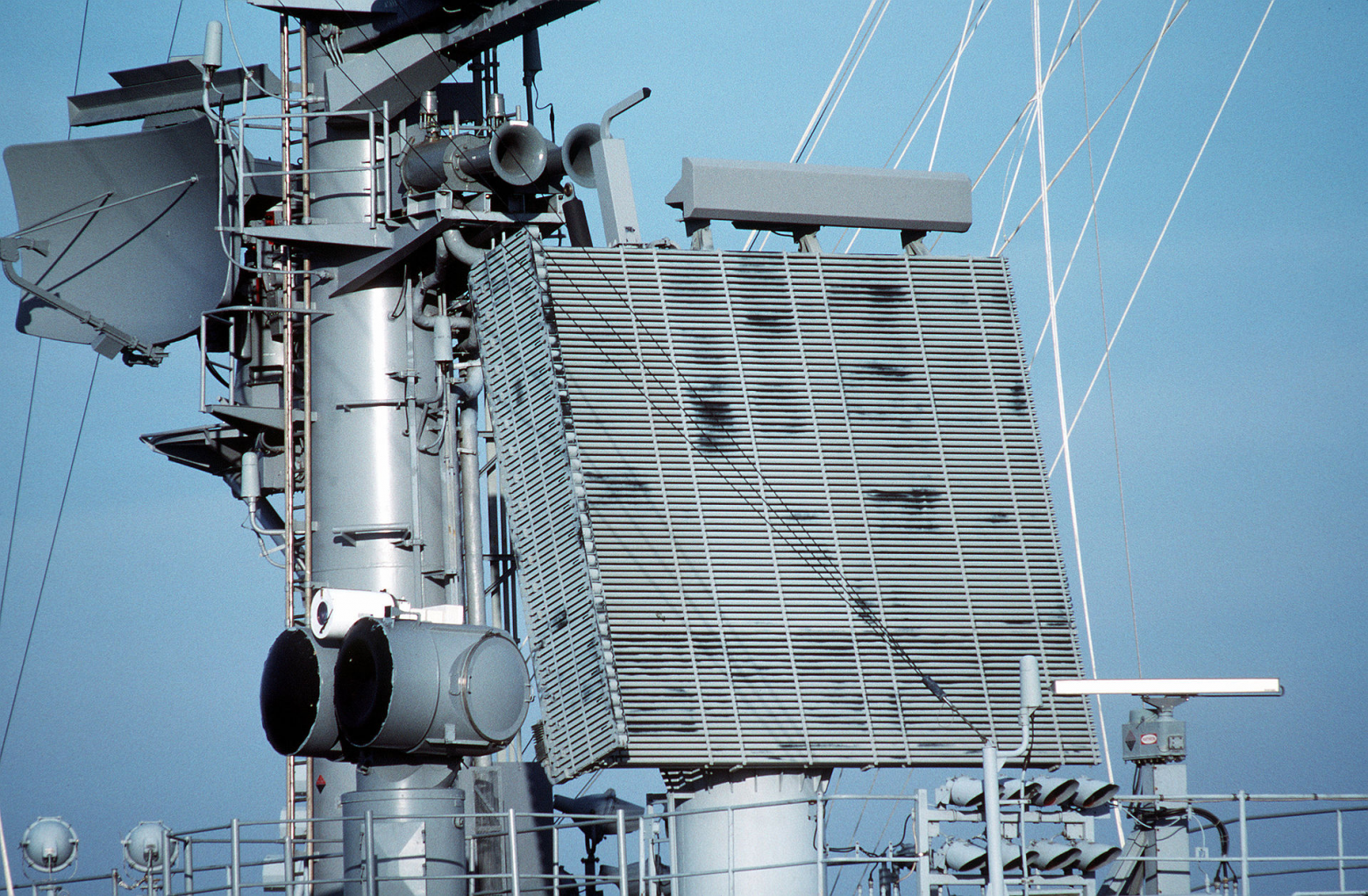
The first PAA to find its embodiment in a non-"stationary" variant was the American AN/SPY-1 system, created as part of the extremely ambitious AEGIS weapons control computer system project. AEGIS combined four PESA SPY-1 arrays looking in different cardinal directions providing all-around coverage, continuously tracked all targets around the ship with them, and automatically distributed those targets among available weapons — from guns to anti-aircraft missiles. Moreover, for compatibility with "old" anti-aircraft missiles with semi-active seekers, AEGIS implemented the scheme already mentioned in this article where the computer controlled launched missiles in radio command mode until the last seconds, automatically activating the illumination radar only immediately before target engagement for precise "final guidance" of the missile. Immediately after the missile's explosion, the illuminator could switch to the next target, and if for some reason this wasn't possible, the missiles could be detonated in radio command mode as well. In theory, the resulting monster could track up to 100 targets and simultaneously control 18 launched anti-aircraft missiles, distributing targets among illumination radars of which Ticonderoga-class ships had 4 and smaller Arleigh Burkes had 3. Add to all this the ability to unite several such ships into a single computer network automatically distributing targets among ships! The first prototype system was launched on an experimental ship in 1973, but practical refinement of such an ambitious system predictably dragged on, and the first combat ship with AEGIS entered service only in 1983.

So Soviet engineers ultimately beat their American colleagues to the practical deployment of PESA in real SAM systems. Ironically, the USSR also launched a very ambitious S-300 project that envisioned creating a single super-system that could replace most other types of SAM systems for both ground forces and ships. But just as with the Americans, the Soviets encountered enormous problems with implementation, which ultimately led to the creation of three completely different SAM systems with minimal degree of unification that, because of the retained similar name, everyone still confuses with each other to this day. The first to be brought to completion was the S-300P complex created for the country's strategic air defense. And like the S-25 several decades before, at the time of its adoption (1978) this complex was indisputably the best and most advanced air defense system in the world.

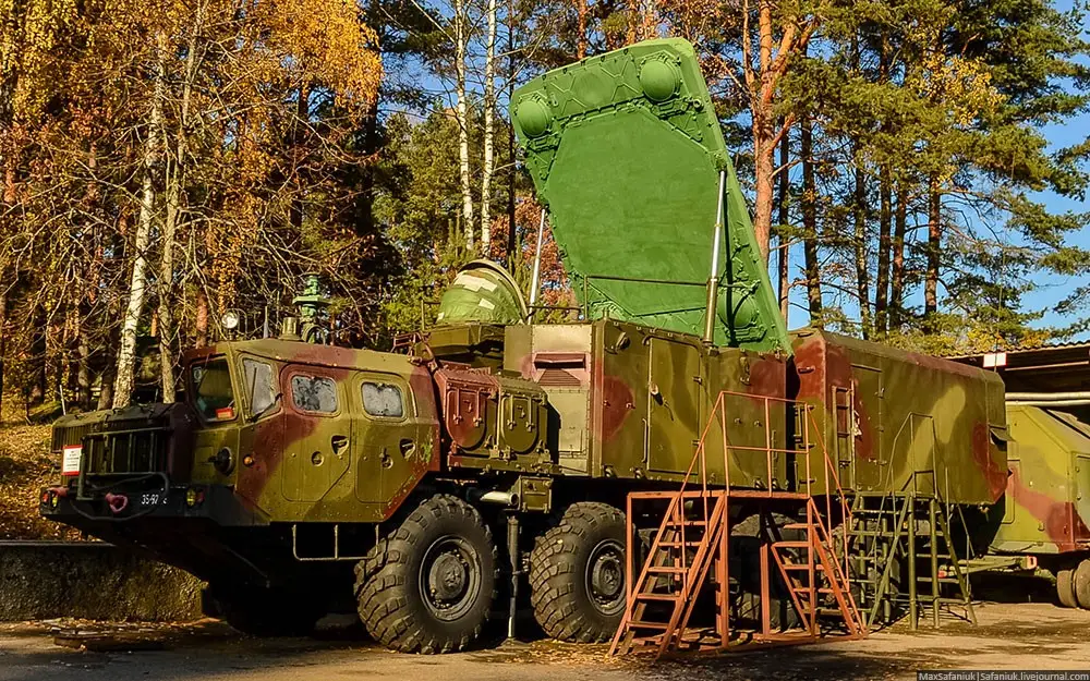
Thanks to PESA, one S-300P battery could simultaneously engage 4 different targets in a 120-degree sector. All vehicles in the complex were self-propelled and easily moved from place to place, evading possible enemy strikes. Moreover, unlike older systems, the S-300 used solid-fuel missiles in hermetically sealed containers that could be stored for decades with almost no maintenance. Well, why am I telling you? This system remains modern even today. However, unlike AEGIS, the SAM system had no separate antennas for "illuminating" the target with a continuous beam and initially could only use 5V55K missiles with simple radio command guidance. This naturally brought back the already-mentioned problem of radio command guidance — at ranges beyond 40 km, target engagement accuracy was quite low, limiting the complex's "range" and effectiveness. However, as the system was refined several years later (1982), the USSR managed to create the 5V55R missile with semi-active homing capable of working with pulsed radar signals.

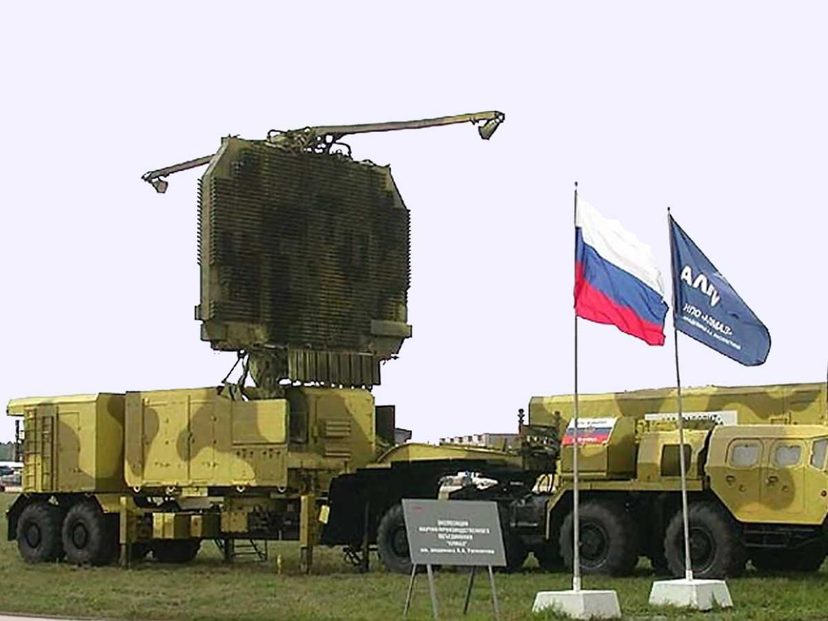
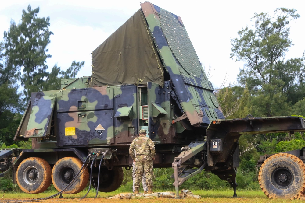
For this, Soviet engineers invented a scheme the Americans call TVM — "track via missile." In this scheme, the missile still retains radio command control but has its own antenna and radar signal receiver that doesn't process the signal itself but retransmits it back to the ground control station. Thus, the ground station effectively gets a mobile radar moving with the missile. The relay scheme is convenient because the missile doesn't need to decode the radar signal or have a complex control system, and the radar doesn't need to illuminate the target continuously. At the same time, nearly all the advantages of semi-active homing for accuracy are preserved and the ability to conduct simultaneous fire at a large number of targets is ensured. The Americans soon (1984) applied a similar scheme with PESA and TVM in their PATRIOT system:

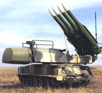
Interestingly, in the "field" S-300V SAM system that was brought to completion around the same time, they didn't bother with TVM and simply mounted a continuous target illumination radar on the launcher. However, as with AEGIS, it only activates for "final guidance" of the missile in the last seconds of flight. Overall, the approach of using several launchers with relatively simple radars instead of one "super-radar" capable of simultaneously engaging several targets apparently appealed more to Soviet military planners. Yes, each such launcher can only fire at one aircraft at a time, but there are 6 of these launchers in a Buk SAM system (for example) per battery. With automated control, receiving external target designation from a central control station, such a battery can also engage 6 aircraft simultaneously by simply distributing targets among different TELARs. Moreover, unlike the S-300P where disabling one radar renders all other vehicles in the battery useless, the Buk remains combat-capable until all 6 launchers are destroyed. However, the S-300P ultimately proved to be the cheaper option and today systems created on its basis are used more often.

Further development of phased array radars became possible only in the 21st century. It was enabled by the development of radio-frequency microelectronics making possible the mass creation of relatively cheap and compact transceivers, and the appearance of computing devices capable of digital signal processing from many thousands of receivers simultaneously. Modern AESAs have two main advantages:

• The ability to simultaneously operate on more than one frequency (for example, simultaneously forming several beams directed in different directions on different frequencies)
• The ability to switch beams "digitally" during reception, forming not one but any number of receive beams

We've already discussed the first advantage of AESA. In the radar context, it simplifies the implementation of "low observable" LPIR schemes that form a complex, "encrypted" signal that the adversary will find difficult to detect. The second advantage of AESA is that the received digital signal can be "stored" and "replayed" any number of times. Since the antenna pattern is formed by digital processing, the same received signal can be processed in a dozen different ways yielding different antenna patterns. In fact, the only limitation here is the radar's computational capacity. A sufficiently advanced AESA can continuously observe all space as essentially a 2D image in a 120x120 degree sector, without needing to choose any specific direction in advance. A PESA can achieve a similar result only through "line-by-line scanning" where the image refresh rate is an order of magnitude lower. This is a major advantage because any pulsed radar transmits only a small fraction of the time while "listening" to the airwaves almost constantly. This allows an AESA radar to send a series of short pulses to several targets simultaneously and then listen for the return signal from all of them at once. A PESA cannot do this — at any given moment it can track only one target, though it can switch between them very quickly. Accordingly, the capabilities for simultaneously tracking large numbers of targets with AESA are an order of magnitude higher.

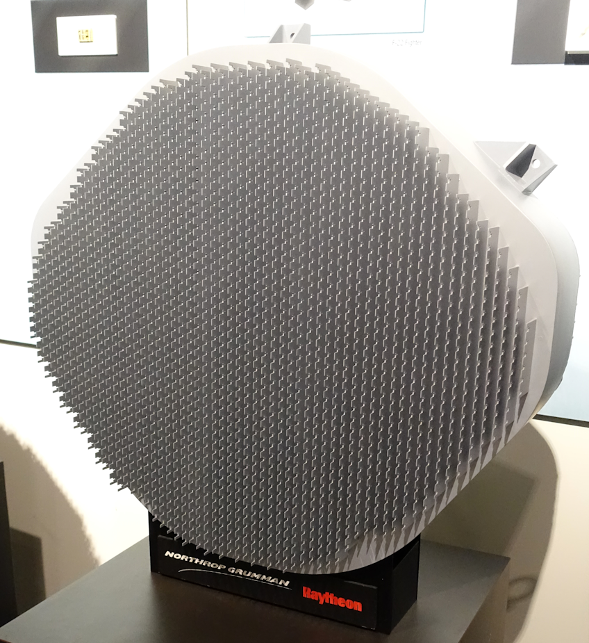
The only disadvantages of AESA are their high price and a fairly "bulky" antenna assembly because it must be built from relatively large transceiver modules with heat dissipation concerns. Radars using PESA may be larger overall, but most of their electronics can be packed into the stationary part while the radiating elements are very compact:

Consequently, PESAs are still frequently encountered in aviation radars where volume is at a premium and every gram counts, while large stationary and naval radars like modern versions of AEGIS are gradually transitioning to AESA. However, it should be remembered that compared to PESA, AESA deployment requires a much greater volume of research and development work. Therefore, many smaller radar manufacturers still don't have an AESA model in their portfolio. Moreover, AESA development requires a country to have well-developed microelectronics in general and microwave integrated electronics in particular. Therefore, despite the relative simplicity of the PAA concept as a whole, in practice AESA creation remains the prerogative of countries with high technological potential.

Another interesting recent trend has been the application of AESA in wideband systems (such as the already-mentioned satellite terminals) and especially in RFI radar (radio frequency identification) systems. These are new systems designed to determine target characteristics not from an echo signal as in conventional radars, but from targets' ability to re-emit electromagnetic waves incident on them. In terms of approach, this is similar to how RFI tags used in supermarkets work ("electronic price tags," anti-theft systems, etc.). The advantage of RFI over conventional radars is the absence of need for powerful transmitting equipment (which simplifies system design). The disadvantage is that targets must carry special active transponders that re-emit the signal incident on them. Therefore, RFI finds application only in systems monitoring marked targets — for example in aviation and maritime where installing a transponder on an object has long been the norm. In the context of radar development, the existence of various systems like ADS-B in aviation and AIS (Automatic Identification System) on ships means the gradual displacement of classic passive radars by active target identification systems.