Discrete Fourier Transform in Living Pictures for Ninth Graders

The goal of this article is not to provide a rigorous mathematical definition of the Fourier transform — countless authors have done that already — but rather to demonstrate its "mechanical" meaning through examples and explain why it works.

You'll need mathematics and physics knowledge at the 9th-grade level: the Pythagorean theorem, sine and cosine definitions in right triangles, and a basic understanding of sinusoids. By the end, we'll apply these concepts to decode telephone numbers from audio files encoded as DTMF signals.

Disclaimer: I explicitly discourage mathematicians and those who prefer formal rigor from reading this. There are no proofs or formal strictness here — only animations, images, analogies, and examples comprehensible to someone with an incomplete secondary education.

Virtual Laboratory Instruments

Two virtual recorders serve as our research tools. They accept signals (for example, electrical voltage) and move a writing mechanism from the zero position proportionally to the signal values.

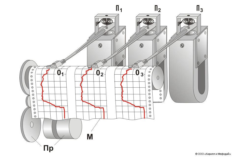
The recorder includes a writing node with a pen (O1, O2, O3) containing ink-saturated porous material and electromechanical drives (P1, P2, P3) that move the pens based on current levels. The paper tape (M) moves at constant speed via the transport mechanism (Pr).

The tape develops the signal over time. Knowing the tape speed, you can determine signal values at any specific moment.

Another recorder variant uses rotating paper circles instead of tape. We'll use both types in our investigations.

First Experiment: Level Zero

Our virtual instruments receive a zero signal. The writing pens settle at the mid-position corresponding to zero input. The tape moves at one division per second. The disk rotates at one sector per second with 12 total sectors.

Both instruments work synchronously. The tape recorder outputs six points per second — this is the measurement and recording speed of our instruments. This digital behavior will become important later.

Second Experiment: A Straight Line

Testing the linear function y = 0.5t shows different results on each instrument. The tape recorder draws a nearly straight line; the circular recorder produces something quite different.

The difference lies only in the paper movement beneath the pens. Both pens make identical movements — the displays differ only because of the different paper movement modes.

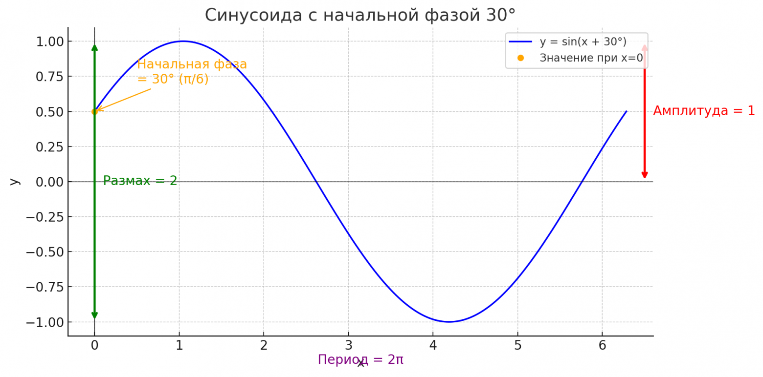
Third Experiment: A Circular Sinusoid

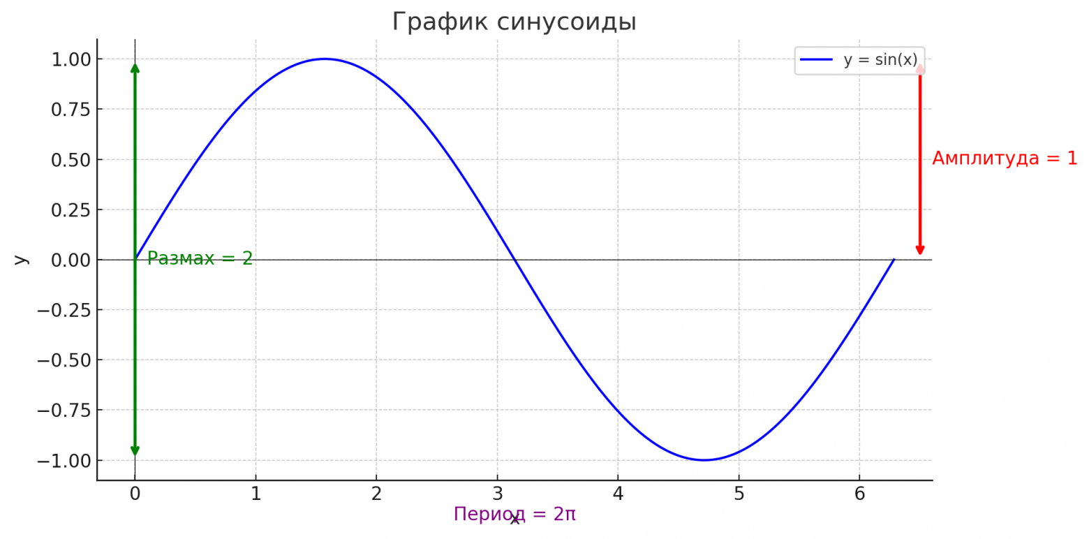
Inputting a sinusoidal signal reveals one complete period (2pi radians or 360 degrees) over 12 divisions of tape, or 12 seconds.

Angular frequency is the rate of argument change per second in sinusoidal functions, measured in radians per second.

Example: A motor rotating 600 times per minute has an angular frequency of 20pi rad/s, or 3600 degrees/s (since 10 rotations per second times 360 degrees = 3600 degrees/s).

The signal formula is: y = A * sin(omega * t + phi)

In this example:

• Amplitude A = 10
• Period T = 12 s
• Frequency v = 1/12 Hz
• Angular frequency omega = 2pi*v = pi/6 rad/s
• Initial phase phi = 0

So: y = 10 * sin(pi/6 * t)

Over t = 12 seconds, the argument (pi/6)*t changes by 2pi radians (360 degrees), after which values repeat. The circular recorder rotates with the same 12-second period, creating a perfect circle.

Key Observation: Point M

A "wandering" point M appears on the circular recorder — the center of mass of all curve points. Its coordinates are calculated as averages:

M_x = (1/N) * SUM(R_xn)
M_y = (1/N) * SUM(R_yn)

Where N is the number of curve points, and R_xn, R_yn are the coordinates of the n-th point.

In physics, this is the center of mass of the mechanical system. More precisely, it represents the complex amplitude of a harmonic (called a "phasor" in English).

• M_x = real part of the complex amplitude
• M_y = imaginary part of the complex amplitude

Important observation: When the input signal's period matches the disk rotation period, point M does not collapse to the origin. When they don't match, M migrates toward (0, 0).

Fourth Experiment: Slowing Down

Slowing the circular recorder to a 24-second rotation period (half speed) while keeping the sinusoid unchanged produces a four-petaled flower pattern. Point M migrates toward the origin.

Slowing further to a 36-second rotation (one-third speed) shows M approaching the origin even more.

Fifth Experiment: Speeding Up

Accelerating to a 6-second rotation period produces similar behavior — point M again seeks zero coordinates.

Why Does Point M Behave This Way?

When periods coincide: Signal maxima and minima occur at identical disk sectors repeatedly, producing symmetrical curves with M remaining offset from the origin.

When periods don't match: Maxima and minima constantly shift position, creating symmetric patterns centered at (0, 0), causing M to approach the origin.

Extracting Information from M's Coordinates

For signals whose period matches the disk rotation:

• The vector length |OM| equals half the amplitude (or one-quarter of the peak-to-peak range)
• The angle between the X-axis and OM equals the signal's phase (interpreted as cosine). For sine interpretation, use the angle between the Y-axis and OM.

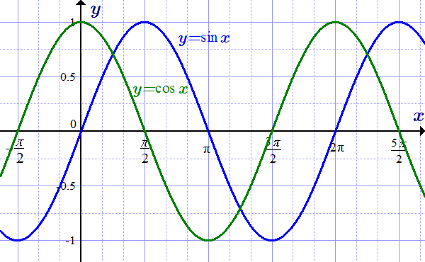
Sine and cosine differ only by a 90-degree phase shift: sin(x) = cos(x - pi/2); cos(x) = sin(x + pi/2)

Vector length calculation (Pythagorean theorem):
|OM| = sqrt(M_x^2 + M_y^2)

Angle calculation:
tan(phi) = M_y / M_x, so phi = arctan(M_y / M_x)

Sixth Experiment: Decomposing Mixed Harmonics

Testing a complex signal: y = 2*sin(omega*t + pi/3) + 4*cos(3*omega*t) + 3*cos(6*omega*t + pi/4)

Where omega = pi/6 rad/s (the 1st harmonic).

Sequential disk rotation at harmonic speeds reveals each component's parameters:

• 1st harmonic: M_d is approximately 1 (amplitude 2), phase approximately 60 degrees — matches expected values
• 2nd harmonic: M approaches 0 — absent, as expected
• 3rd harmonic: M_d is approximately 2 (amplitude 4), zero phase — matches the cosine without phase shift
• 4th and 5th harmonics: Confirmed absent
• 6th harmonic: M_d is approximately 1.5 (amplitude 3), angle approximately 45 degrees — matches specifications

Note: Accuracy decreases for higher harmonics due to fewer data points per period.

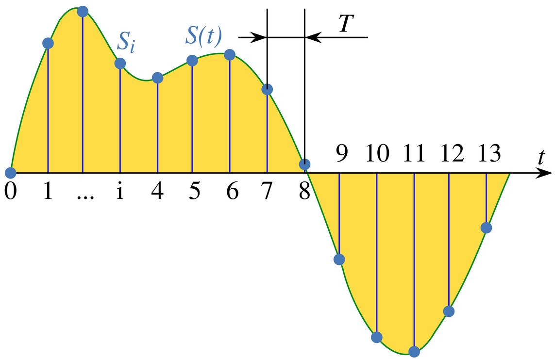
What Is a Sample?

A sample is a numerical signal value at a specific moment. CD Audio uses 44,100 sixteen-bit samples per second per channel.

• One second of CD audio = 2 channels * 44,100 samples = 88,200 samples = 176,400 bytes
• 0.1 seconds of CD mono = 4,410 sixteen-bit numbers

Seventh Experiment: Offset Sine and the Zero Harmonic

Testing: y = 4 + 6*sin(pi/6 * t)

The DC offset affects the circular pattern — it's no longer a perfect circle. Yet vector M_d still approaches 3 (half the amplitude of 6), with zero phase — as if the offset doesn't exist.

To determine the offset constant (4), construct the zero harmonic by stopping the disk rotation:

M_d approaches 4 — which is the mean value of the function.

Key finding: The zero harmonic's M_d length equals the average of the entire function.

Placing Signal Samples on the Circular Graph

Samples (discrete measurements from an ADC) must be positioned on the circular graph. Each sample has a value r and a phase alpha.

Phase calculation:

alpha = 360 * k * (n/N) [in degrees]
alpha = 2*pi * k * (n/N) [in radians]

Where:

• k = harmonic number
• n = sample index (0 to N-1)
• N = total samples in the analysis window

The fraction n/N scales the sample position to [0, 1), then multiplication by 360 degrees (or 2pi) converts to an angle. The harmonic multiplier k scales the angle so that one k-th harmonic period occupies the full 360-degree rotation.

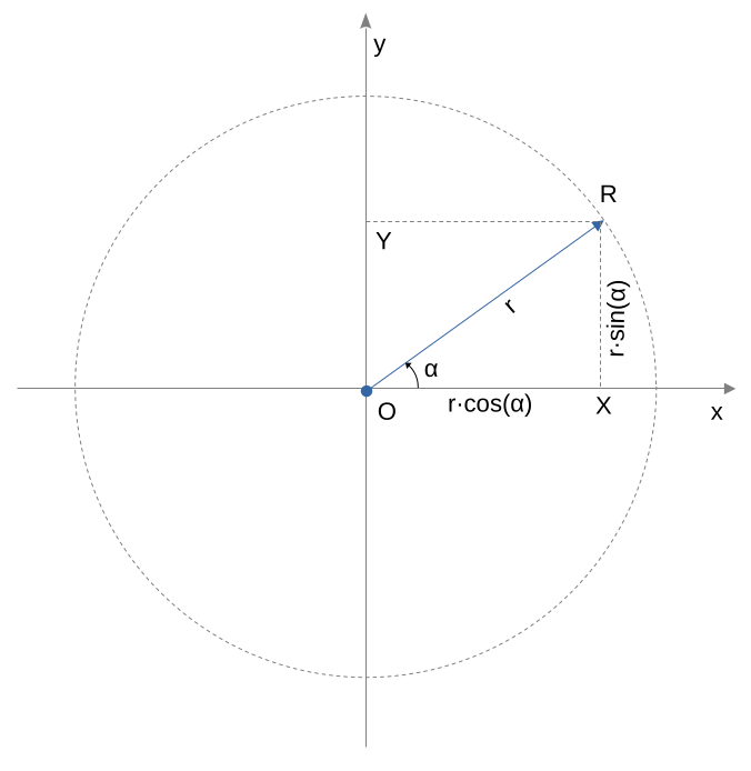
Sample Coordinates on the Circular Graph

Given angle alpha and sample value r, convert from polar to Cartesian coordinates:

R_x = r * cos(alpha)
R_y = r * sin(alpha)

Substituting alpha = 2*pi*k*n/N:

R_x(k) = r_n * cos(2*pi*k*n/N)
R_y(k) = r_n * sin(2*pi*k*n/N)

Where r_n is the n-th sample's magnitude, k is the harmonic number, n is the sample index, and N is the total number of samples.

The Discrete Fourier Transform

Using the mean point M formula and substituting our coordinate expressions:

M_x(k) = (1/N) * SUM from n=0 to N-1 of: r_n * cos(2*pi*k*n/N)

M_y(k) = (1/N) * SUM from n=0 to N-1 of: r_n * sin(2*pi*k*n/N)

Where:

• M_x(k) = real part of the k-th harmonic's complex amplitude
• M_y(k) = imaginary part of the k-th harmonic's complex amplitude
• N = number of samples in the analysis window
• r_n = n-th sample value
• k = harmonic number (0 to N-1)

These paired formulas constitute the Discrete Fourier Transform (DFT).

Practical Application: Decoding Telephone Numbers from Audio

DTMF (Dual-Tone Multi-Frequency) signaling replaced pulse dialing with faster, more reliable two-tone transmission. It was widely deployed in former Soviet telephone networks from the mid-1990s.

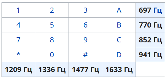
DTMF encodes digits 0-9, symbols *, #, and letters A-D as pairs of specific frequencies:

• 697/1209 Hz = '1', 697/1336 Hz = '2', 697/1477 Hz = '3', 697/1633 Hz = 'A'
• 770/1209 Hz = '4', 770/1336 Hz = '5', 770/1477 Hz = '6', 770/1633 Hz = 'B'
• 852/1209 Hz = '7', 852/1336 Hz = '8', 852/1477 Hz = '9', 852/1633 Hz = 'C'
• 941/1209 Hz = '*', 941/1336 Hz = '0', 941/1477 Hz = '#', 941/1633 Hz = 'D'

Our test file is converted from a Wikipedia DTMF recording (8000 samples/s, 8-bit PCM). It contains 8 ten-digit phone numbers: 0696675356, 4646415180, 2336731416, 3608338160, 4400826146, 6253689638, 8482138178, 5073643399.

Determining Requirements

The closest DTMF frequencies (697 and 770 Hz) differ by 73 Hz — this is the minimum required resolution. We double it to 35 Hz for reliability against spectral leakage.

Spectral leakage occurs when the analysis window doesn't contain an integer number of periods of the investigated harmonic.

Buffer size: N = SampleRate / v1 = 8000 / 35 = 228.57, rounded to 228 samples.

Adjusted resolution: v1 = 8000 / 228 = 35.1 Hz

Frequency-to-Harmonic Mapping

Each DTMF frequency maps to a harmonic number:

• 697 Hz -> harmonic 20 (round(697/35.1))
• 770 Hz -> harmonic 22
• 852 Hz -> harmonic 24
• 941 Hz -> harmonic 27
• 1209 Hz -> harmonic 34
• 1336 Hz -> harmonic 38
• 1477 Hz -> harmonic 42
• 1633 Hz -> harmonic 47

DTMF frequencies rarely align exactly with harmonics — some fall between them. This justifies our choice of 35 Hz resolution.

Python Implementation

import math as m

# DTMF harmonic resolution.
harmonic_resolution = 35  # 35 Hz per harmonic
# Sample rate.
sample_rate = 8000  # 8000 samples per second
# Harmonic detection magnitude.
harmonic_detection_magnitude = 5
# Calculate the number of samples per chunk.
N = sample_rate // harmonic_resolution  # 8000 / 35 = 228 samples per chunk
# Recalculate the harmonic resolution to be the actual value.
harmonic_resolution = sample_rate / N  # 8000 / 228 = 35.09 Hz
# Calculate the number of samples per shift.
shift_interval = N // 3  # 228 / 3 = 76 samples per shift
# Silence between whole phone numbers is 0.2 seconds.
silence_interval = 0.2
# Calculate the number of iterations for the silence interval.
silence_number = round(silence_interval / (shift_interval / sample_rate))

# DTMF frequencies.
dtmf_frequencies = [697, 770, 852, 941, 1209, 1336, 1477, 1633]
# DTMF digits to frequency mapping.
freq_to_digit = {
     (697, 1209): '1', (697, 1336): '2', (697, 1477): '3', (697, 1633): 'A',
     (770, 1209): '4', (770, 1336): '5', (770, 1477): '6', (770, 1633): 'B',
     (852, 1209): '7', (852, 1336): '8', (852, 1477): '9', (852, 1633): 'C',
     (941, 1209): '*', (941, 1336): '0', (941, 1477): '#', (941, 1633): 'D'
}

def get_harmonic(frequency: int) -> int:
    return round(frequency / harmonic_resolution)

dtmf_harmonics = [get_harmonic(f) for f in dtmf_frequencies]

harmonic_to_digit = {
    (get_harmonic(d[0]), get_harmonic(d[1])): h
    for d, h in freq_to_digit.items()
}

def get_digit(harmonic1: int, harmonic2: int) -> str:
    h = (min(harmonic1, harmonic2), max(harmonic1, harmonic2))
    return harmonic_to_digit.get(h)

def get_frequency(k):
    return k * harmonic_resolution

def get_magnitude(phase_vector: dict) -> float:
    re = phase_vector['re']
    im = phase_vector['im']
    return m.sqrt(re * re + im * im)

def calculate_dft(data: list[int], harmonics: list[int]) -> list[dict]:
    dft = [None] * len(harmonics)
    for i in range(len(harmonics)):
        k = harmonics[i]
        sum_x = 0.0
        sum_y = 0.0
        for n in range(N):
            r = data[n]
            x = r * m.cos(2 * m.pi * k * n / N)
            y = r * m.sin(2 * m.pi * k * n / N)
            sum_x += x
            sum_y += y
        sum_x /= N
        sum_y /= N
        dft[i] = {'re': sum_x, 'im': sum_y}
    return dft

samples = []
found_dtmf = False
silence_counter = 0

with open("dtmf.wav", "rb") as f:
    f.seek(44)  # Skip WAV header
    while (byte := f.read(1)):
        samples.append(byte[0])
        if len(samples) == N:
            dft = calculate_dft(samples, dtmf_harmonics)
            magnitudes_per_harmonic = {}
            for i in range(len(dft)):
                phase_vector = dft[i]
                magnitude = get_magnitude(phase_vector)
                magnitudes_per_harmonic[dtmf_harmonics[i]] = magnitude
            sorted_harmonics = [
                {'k': item[0], 'm': item[1]}
                for item in sorted(
                    magnitudes_per_harmonic.items(),
                    key=lambda item: item[1],
                    reverse=True
                )[:2]
            ]
            if (len(sorted_harmonics) == 2 and
                sorted_harmonics[0]['m'] > harmonic_detection_magnitude and
                sorted_harmonics[1]['m'] > harmonic_detection_magnitude):
                digit = get_digit(
                    sorted_harmonics[0]['k'],
                    sorted_harmonics[1]['k']
                )
                if digit:
                    silence_counter = 0
                    if not found_dtmf:
                        print(digit, end="")
                        found_dtmf = True
                else:
                    print("?", end="")
            else:
                found_dtmf = False
                silence_counter += 1

            if silence_counter == silence_number:
                print("")

            samples = samples[shift_interval:]

Implementation Details

Buffer accumulation trade-off: 228 samples equals 28.5 milliseconds. Larger buffers improve accuracy but increase latency. Real-time applications must balance these concerns.

DTMF duration standard: ETSI ES 201 235-3 specifies a minimum of 40 ms for reliable recognition. Our 28.5 ms buffer should suffice.

Sliding window approach: The signal may not start at the buffer's beginning. Shifting the window by one-third (76 samples) ensures detection regardless of alignment. This means the same symbol may be detected across multiple windows.

Duplicate prevention: The found_dtmf flag prevents outputting the same symbol multiple times. It resets only after detecting silence on the DTMF harmonics.

Execution Results

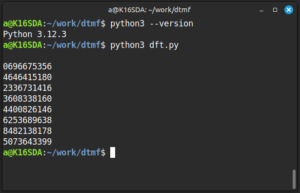
The program reads dtmf.wav and outputs the detected DTMF-encoded telephone numbers, one per line.

Conclusion

This article aims for accessibility over rigor. The simulator and example development required approximately two weeks of evening work. Visualization was prioritized over formal mathematics — the animations and images explain the DFT's mechanisms in a way that's comprehensible without strict proofs.

Code repository: github.com/galilov/DFTDemo